

Soft Degrees of Freedom, Gibbons–Hawking Contribution and Entropy from. . .
377
partition functions (without zero modes). In the latter, we thus consider expansions
as in equation (4.4) of [25], with d = 3 and p = 1, but we explicitly keep the
zero mode because we need it for the microscopic understanding of the Gibbons–
Hawking contribution. This is reminiscent of the expansion of the complex scalar
field in [26].
6 Dynamics and Charge
For the transverse degrees of freedom at k 3 = 0, the usual discussion in terms of
two transverse polarizations applies. In addition, the canonical Hamiltonian H 0 =
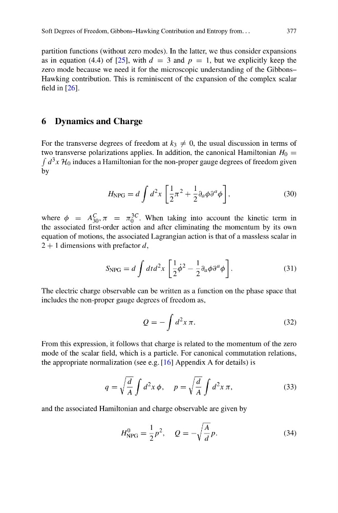
d 3 x H 0 induces a Hamiltonian for the non-proper gauge degrees of freedom given
by
H NPG = d
d
2 x
1
2
π
2
+
1
2
∂ a φ∂
a φ
,
(30)
where φ = A C
30 , π = π 3C
0 . When taking into account the kinetic term in
the associated first-order action and after eliminating the momentum by its own
equation of motions, the associated Lagrangian action is that of a massless scalar in
2 + 1 dimensions with prefactor d,
S NPG = d
dtd
2 x
1
2
˙
φ
2
−
1
2
∂ a φ∂
a φ
.
(31)
The electric charge observable can be written as a function on the phase space that
includes the non-proper gauge degrees of freedom as,
Q = −
d
2 x π.
(32)
From this expression, it follows that charge is related to the momentum of the zero
mode of the scalar field, which is a particle. For canonical commutation relations,
the appropriate normalization (see e.g. [16] Appendix A for details) is
q =
d
A
d
2 x φ, p =
d
A
d
2 x π,
(33)
and the associated Hamiltonian and charge observable are given by
H
0
NPG =
1
2
p
2 , Q = −
A
d
p.
(34)
377
partition functions (without zero modes). In the latter, we thus consider expansions
as in equation (4.4) of [25], with d = 3 and p = 1, but we explicitly keep the
zero mode because we need it for the microscopic understanding of the Gibbons–
Hawking contribution. This is reminiscent of the expansion of the complex scalar
field in [26].
6 Dynamics and Charge
For the transverse degrees of freedom at k 3 = 0, the usual discussion in terms of
two transverse polarizations applies. In addition, the canonical Hamiltonian H 0 =
d 3 x H 0 induces a Hamiltonian for the non-proper gauge degrees of freedom given
by
H NPG = d
d
2 x
1
2
π
2
+
1
2
∂ a φ∂
a φ
,
(30)
where φ = A C
30 , π = π 3C
0 . When taking into account the kinetic term in
the associated first-order action and after eliminating the momentum by its own
equation of motions, the associated Lagrangian action is that of a massless scalar in
2 + 1 dimensions with prefactor d,
S NPG = d
dtd
2 x
1
2
˙
φ
2
−
1
2
∂ a φ∂
a φ
.
(31)
The electric charge observable can be written as a function on the phase space that
includes the non-proper gauge degrees of freedom as,
Q = −
d
2 x π.
(32)
From this expression, it follows that charge is related to the momentum of the zero
mode of the scalar field, which is a particle. For canonical commutation relations,
the appropriate normalization (see e.g. [16] Appendix A for details) is
q =
d
A
d
2 x φ, p =
d
A
d
2 x π,
(33)
and the associated Hamiltonian and charge observable are given by
H
0
NPG =
1
2
p
2 , Q = −
A
d
p.
(34)