

354
S. S. Roy et al.
1
2
3
4
5
6
7
i
0
0.2
0.4
0.6
0.01
6
1 0
1 4
0.012
0.014
E
N
1
2
3
4
5
6
i
0.1
0.2
0.3
0.4
b
a
s A (i)
s A (i)
=0.2
=0.6
=1.0
=2.0
=4.0
6
8
10
12
0
0.02
0.04
0.06
E
N
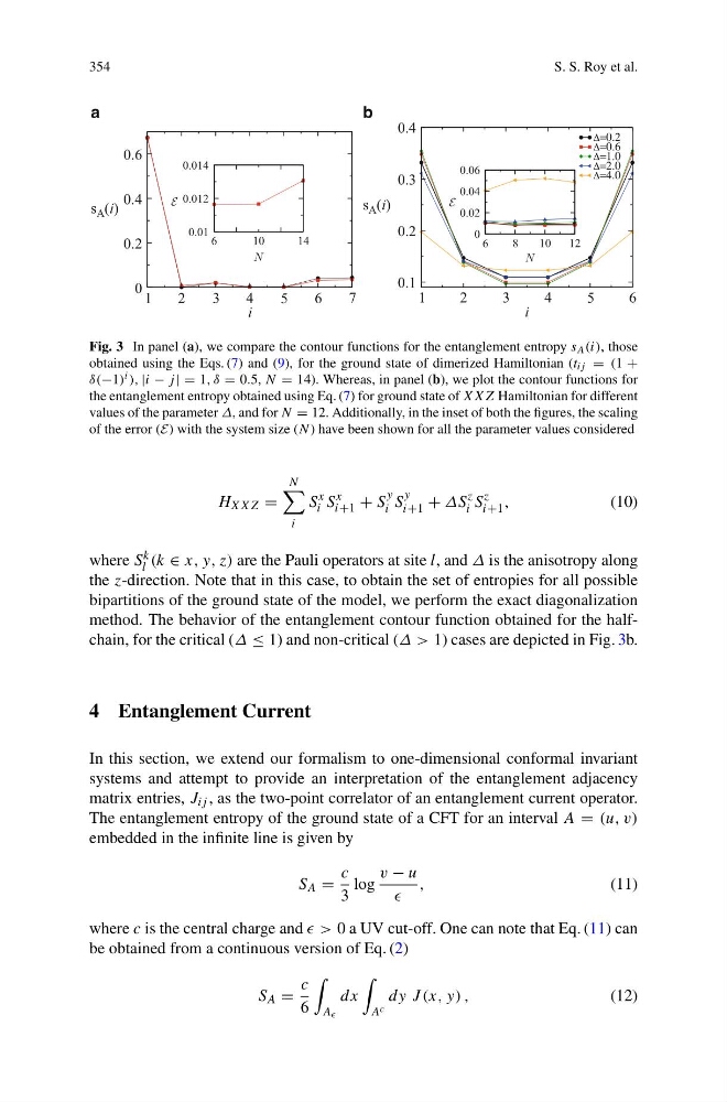
Fig. 3 In panel (a), we compare the contour functions for the entanglement entropy s A (i), those
obtained using the Eqs. (7) and (9), for the ground state of dimerized Hamiltonian (t ij = (1 +
δ(−1) i ), |i − j | = 1, δ = 0.5, N = 14). Whereas, in panel (b), we plot the contour functions for
the entanglement entropy obtained using Eq. (7) for ground state of XXZ Hamiltonian for different
values of the parameter Δ, and for N = 12. Additionally, in the inset of both the figures, the scaling
of the error (E) with the system size (N ) have been shown for all the parameter values considered
H XXZ =
N
i
S
x
i S
x
i+1 + S
y
i S
y
i+1 + ΔS
z
i S
z
i+1 ,
(10)
where S k
l (k ∈ x, y, z) are the Pauli operators at site l, and Δ is the anisotropy along
the z-direction. Note that in this case, to obtain the set of entropies for all possible
bipartitions of the ground state of the model, we perform the exact diagonalization
method. The behavior of the entanglement contour function obtained for the halfchain, for the critical (Δ ≤ 1) and non-critical (Δ > 1) cases are depicted in Fig. 3b.
4 Entanglement Current
In this section, we extend our formalism to one-dimensional conformal invariant
systems and attempt to provide an interpretation of the entanglement adjacency
matrix entries, J ij , as the two-point correlator of an entanglement current operator.
The entanglement entropy of the ground state of a CFT for an interval A = (u, v)
embedded in the infinite line is given by
S A =
c
3
log
v − u
,
(11)
where c is the central charge and > 0 a UV cut-off. One can note that Eq. (11) can
be obtained from a continuous version of Eq. (2)
S A =
c
6
A
dx
A c
dy J (x, y) ,
(12)
S. S. Roy et al.
1
2
3
4
5
6
7
i
0
0.2
0.4
0.6
0.01
6
1 0
1 4
0.012
0.014
E
N
1
2
3
4
5
6
i
0.1
0.2
0.3
0.4
b
a
s A (i)
s A (i)
=0.2
=0.6
=1.0
=2.0
=4.0
6
8
10
12
0
0.02
0.04
0.06
E
N
Fig. 3 In panel (a), we compare the contour functions for the entanglement entropy s A (i), those
obtained using the Eqs. (7) and (9), for the ground state of dimerized Hamiltonian (t ij = (1 +
δ(−1) i ), |i − j | = 1, δ = 0.5, N = 14). Whereas, in panel (b), we plot the contour functions for
the entanglement entropy obtained using Eq. (7) for ground state of XXZ Hamiltonian for different
values of the parameter Δ, and for N = 12. Additionally, in the inset of both the figures, the scaling
of the error (E) with the system size (N ) have been shown for all the parameter values considered
H XXZ =
N
i
S
x
i S
x
i+1 + S
y
i S
y
i+1 + ΔS
z
i S
z
i+1 ,
(10)
where S k
l (k ∈ x, y, z) are the Pauli operators at site l, and Δ is the anisotropy along
the z-direction. Note that in this case, to obtain the set of entropies for all possible
bipartitions of the ground state of the model, we perform the exact diagonalization
method. The behavior of the entanglement contour function obtained for the halfchain, for the critical (Δ ≤ 1) and non-critical (Δ > 1) cases are depicted in Fig. 3b.
4 Entanglement Current
In this section, we extend our formalism to one-dimensional conformal invariant
systems and attempt to provide an interpretation of the entanglement adjacency
matrix entries, J ij , as the two-point correlator of an entanglement current operator.
The entanglement entropy of the ground state of a CFT for an interval A = (u, v)
embedded in the infinite line is given by
S A =
c
3
log
v − u
,
(11)
where c is the central charge and > 0 a UV cut-off. One can note that Eq. (11) can
be obtained from a continuous version of Eq. (2)
S A =
c
6
A
dx
A c
dy J (x, y) ,
(12)