

352
S. S. Roy et al.
the value of the constant term in Eq. (2), s 0 = log(2). This suggests that the
GHZ state does not have a geometrical interpretation in this framework.
2.3 Numerical Computation
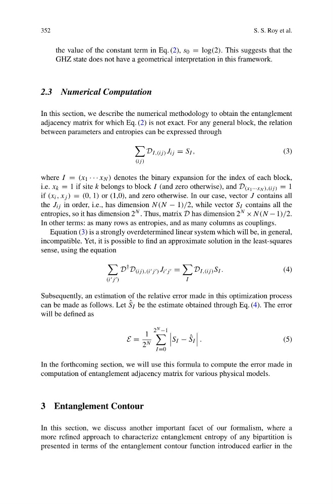
In this section, we describe the numerical methodology to obtain the entanglement
adjacency matrix for which Eq. (2) is not exact. For any general block, the relation
between parameters and entropies can be expressed through
(ij )
D I,(ij ) J ij = S I ,
(3)
where I = (x 1 · · · x N ) denotes the binary expansion for the index of each block,
i.e. x k = 1 if site k belongs to block I (and zero otherwise), and D (x 1 ···x N ),(ij ) = 1
if (x i , x j ) = (0, 1) or (1,0), and zero otherwise. In our case, vector J contains all
the J ij in order, i.e., has dimension N(N − 1)/2, while vector S I contains all the
entropies, so it has dimension 2 N . Thus, matrix D has dimension 2 N × N(N − 1)/2.
In other terms: as many rows as entropies, and as many columns as couplings.
Equation (3) is a strongly overdetermined linear system which will be, in general,
incompatible. Yet, it is possible to find an approximate solution in the least-squares
sense, using the equation
(i j )
D
†
D (ij ),(i j ) J i j =
I
D I,(ij ) S I .
(4)
Subsequently, an estimation of the relative error made in this optimization process
can be made as follows. Let ˆ
S I be the estimate obtained through Eq. (4). The error
will be defined as
E =
1
2 N
2 N −1
I =0
SI − ˆ
S I
.
(5)
In the forthcoming section, we will use this formula to compute the error made in
computation of entanglement adjacency matrix for various physical models.
3 Entanglement Contour
In this section, we discuss another important facet of our formalism, where a
more refined approach to characterize entanglement entropy of any bipartition is
presented in terms of the entanglement contour function introduced earlier in the
S. S. Roy et al.
the value of the constant term in Eq. (2), s 0 = log(2). This suggests that the
GHZ state does not have a geometrical interpretation in this framework.
2.3 Numerical Computation
In this section, we describe the numerical methodology to obtain the entanglement
adjacency matrix for which Eq. (2) is not exact. For any general block, the relation
between parameters and entropies can be expressed through
(ij )
D I,(ij ) J ij = S I ,
(3)
where I = (x 1 · · · x N ) denotes the binary expansion for the index of each block,
i.e. x k = 1 if site k belongs to block I (and zero otherwise), and D (x 1 ···x N ),(ij ) = 1
if (x i , x j ) = (0, 1) or (1,0), and zero otherwise. In our case, vector J contains all
the J ij in order, i.e., has dimension N(N − 1)/2, while vector S I contains all the
entropies, so it has dimension 2 N . Thus, matrix D has dimension 2 N × N(N − 1)/2.
In other terms: as many rows as entropies, and as many columns as couplings.
Equation (3) is a strongly overdetermined linear system which will be, in general,
incompatible. Yet, it is possible to find an approximate solution in the least-squares
sense, using the equation
(i j )
D
†
D (ij ),(i j ) J i j =
I
D I,(ij ) S I .
(4)
Subsequently, an estimation of the relative error made in this optimization process
can be made as follows. Let ˆ
S I be the estimate obtained through Eq. (4). The error
will be defined as
E =
1
2 N
2 N −1
I =0
SI − ˆ
S I
.
(5)
In the forthcoming section, we will use this formula to compute the error made in
computation of entanglement adjacency matrix for various physical models.
3 Entanglement Contour
In this section, we discuss another important facet of our formalism, where a
more refined approach to characterize entanglement entropy of any bipartition is
presented in terms of the entanglement contour function introduced earlier in the