

266
D. O. Campa et al.
the second-order SUSY QM to study the electron motion in bilayer graphene, by
looking for exact solutions to the auxiliary Schrödinger problems.
2 Bilayer Graphene: A Brief Overview
2.1 Effective Hamiltonian
In the study of the electron motion in bilayer graphene, it is usual to work in the
framework of the tight-binding model [1], in which the effective Hamiltonian is
given by
H =
1
2m ∗
0 π 2
(π † ) 2 0
,
(1)
where π = p x − ip y , with p j being the momentum operator in j -direction,
j = x, y. Some important physical quantities are the effective mass of the electron
m ∗ = |t ⊥ |/2v F
2 ≈ 0.054m e , with m e being the free mass electron, the Fermi
velocity v F =
√
3a/2 ¯
h ≈ c/300 where c is the speed of light [2]. Several structure
parameters of the graphene lattice appear as well in the Hamiltonian, e.g., the lattice
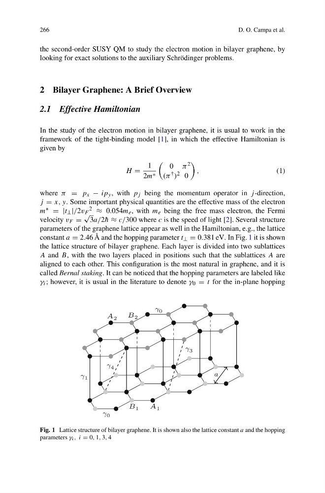
constant a = 2.46 Å and the hopping parameter t ⊥ = 0.381 eV. In Fig. 1 it is shown
the lattice structure of bilayer graphene. Each layer is divided into two sublattices
A and B, with the two layers placed in positions such that the sublattices A are
aligned to each other. This configuration is the most natural in graphene, and it is
called Bernal staking. It can be noticed that the hopping parameters are labeled like
γ i ; however, it is usual in the literature to denote γ 0 = t for the in-plane hopping
B 1
A 1
A 2
B 2
γ 1
γ 0
γ 0
γ 4
γ 3
a
Fig. 1 Lattice structure of bilayer graphene. It is shown also the lattice constant a and the hopping
parameters γ i , i = 0, 1, 3, 4
D. O. Campa et al.
the second-order SUSY QM to study the electron motion in bilayer graphene, by
looking for exact solutions to the auxiliary Schrödinger problems.
2 Bilayer Graphene: A Brief Overview
2.1 Effective Hamiltonian
In the study of the electron motion in bilayer graphene, it is usual to work in the
framework of the tight-binding model [1], in which the effective Hamiltonian is
given by
H =
1
2m ∗
0 π 2
(π † ) 2 0
,
(1)
where π = p x − ip y , with p j being the momentum operator in j -direction,
j = x, y. Some important physical quantities are the effective mass of the electron
m ∗ = |t ⊥ |/2v F
2 ≈ 0.054m e , with m e being the free mass electron, the Fermi
velocity v F =
√
3a/2 ¯
h ≈ c/300 where c is the speed of light [2]. Several structure
parameters of the graphene lattice appear as well in the Hamiltonian, e.g., the lattice
constant a = 2.46 Å and the hopping parameter t ⊥ = 0.381 eV. In Fig. 1 it is shown
the lattice structure of bilayer graphene. Each layer is divided into two sublattices
A and B, with the two layers placed in positions such that the sublattices A are
aligned to each other. This configuration is the most natural in graphene, and it is
called Bernal staking. It can be noticed that the hopping parameters are labeled like
γ i ; however, it is usual in the literature to denote γ 0 = t for the in-plane hopping
B 1
A 1
A 2
B 2
γ 1
γ 0
γ 0
γ 4
γ 3
a
Fig. 1 Lattice structure of bilayer graphene. It is shown also the lattice constant a and the hopping
parameters γ i , i = 0, 1, 3, 4