

NCG and the Batalin–Vilkovisky Construction
251
where, for now, M a , C j , and E are all treated as real variables;
• the self-adjoint linear operator D BV acting on H BV is given by
D BV :=
⎛
⎝
0 R T
R S 0
T 0 0
⎞
⎠
where the linear operators R, S, T are defined by
R : H C → H M ;
ϕ C → [β, ϕ C ],
S : H C → H C ;
ϕ C → [α, ϕ C ],
T : H M → H M ;
ϕ C → [α, ϕ C ] + .
Here, α and β denote Hermitian, traceless 2×2-matrices and we stress that, while
R and S are defined as a commutator, T is an odd derivation, given in terms the
anti-commutator. Alternatively, if we write α and β in terms of the Pauli matrices
as follows:
α =
1
2
(−C
∗
1 )σ 1 + (−C
∗
2 )σ 2 + (−C
∗
3 )σ 3
β =
1
2
(−M
∗
1 )σ 1 + (−M
∗
2 )σ 2 + (−M
∗
3 )σ 3
,
for C ∗
i and M ∗
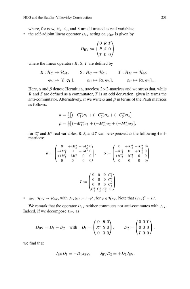
i real variables, R, S, and T can be expressed as the following 4 × 4matrices:
R :=
⎛
⎜
⎜
⎝
0 +iM ∗
3 −iM ∗
2 0
−iM ∗
3
0 +iM ∗
1 0
+iM ∗
2 −iM ∗
1
0 0
0
0
0 0
⎞
⎟
⎟
⎠ ,
S:=
⎛
⎜
⎜
⎝
0 +iC ∗
3 −iC ∗
2 0
−iC ∗
3
0 +iC ∗
1 0
+iC ∗
2 −iC ∗
1
0 0
0
0
0 0
⎞
⎟
⎟
⎠
T :=
⎛
⎜
⎜
⎝
0 0 0 C ∗
1
0 0 0 C ∗
2
0 0 0 C ∗
3
C ∗
1 C ∗
2 C ∗
3 0
⎞
⎟
⎟
⎠
• J BV : H BV → H BV , with J BV (ϕ) := i · ϕ ∗ , for ϕ ∈ H BV . Note that (J BV ) 2 = I d.
We remark that the operator D BV neither commutes nor anti-commutes with J BV .
Indeed, if we decompose D BV as
D BV = D 1 + D 2 with D 1 =
⎛
⎝
0 R 0
R ∗ S 0
0 0 0
⎞
⎠ ,
D 2 =
⎛
⎝
0 0 T
0 0 0
T 0 0
⎞
⎠ .
we find that
J BV D 1 = −D 1 J BV ,
J BV D 2 = +D 2 J BV .
251
where, for now, M a , C j , and E are all treated as real variables;
• the self-adjoint linear operator D BV acting on H BV is given by
D BV :=
⎛
⎝
0 R T
R S 0
T 0 0
⎞
⎠
where the linear operators R, S, T are defined by
R : H C → H M ;
ϕ C → [β, ϕ C ],
S : H C → H C ;
ϕ C → [α, ϕ C ],
T : H M → H M ;
ϕ C → [α, ϕ C ] + .
Here, α and β denote Hermitian, traceless 2×2-matrices and we stress that, while
R and S are defined as a commutator, T is an odd derivation, given in terms the
anti-commutator. Alternatively, if we write α and β in terms of the Pauli matrices
as follows:
α =
1
2
(−C
∗
1 )σ 1 + (−C
∗
2 )σ 2 + (−C
∗
3 )σ 3
β =
1
2
(−M
∗
1 )σ 1 + (−M
∗
2 )σ 2 + (−M
∗
3 )σ 3
,
for C ∗
i and M ∗
i real variables, R, S, and T can be expressed as the following 4 × 4matrices:
R :=
⎛
⎜
⎜
⎝
0 +iM ∗
3 −iM ∗
2 0
−iM ∗
3
0 +iM ∗
1 0
+iM ∗
2 −iM ∗
1
0 0
0
0
0 0
⎞
⎟
⎟
⎠ ,
S:=
⎛
⎜
⎜
⎝
0 +iC ∗
3 −iC ∗
2 0
−iC ∗
3
0 +iC ∗
1 0
+iC ∗
2 −iC ∗
1
0 0
0
0
0 0
⎞
⎟
⎟
⎠
T :=
⎛
⎜
⎜
⎝
0 0 0 C ∗
1
0 0 0 C ∗
2
0 0 0 C ∗
3
C ∗
1 C ∗
2 C ∗
3 0
⎞
⎟
⎟
⎠
• J BV : H BV → H BV , with J BV (ϕ) := i · ϕ ∗ , for ϕ ∈ H BV . Note that (J BV ) 2 = I d.
We remark that the operator D BV neither commutes nor anti-commutes with J BV .
Indeed, if we decompose D BV as
D BV = D 1 + D 2 with D 1 =
⎛
⎝
0 R 0
R ∗ S 0
0 0 0
⎞
⎠ ,
D 2 =
⎛
⎝
0 0 T
0 0 0
T 0 0
⎞
⎠ .
we find that
J BV D 1 = −D 1 J BV ,
J BV D 2 = +D 2 J BV .