

150
D. Levi et al.
However, some reductions cannot be obtained by just studying the Lie point
symmetries of the equation, as was shown in [5] for the Boussinesq equation.
Additional reductions and new solutions can be obtained by considering conditional
symmetries [2], as done in [11]. Many articles are dedicated to this class of
symmetries, for example [17]. To find conditional symmetries of the given PDE, one
adds a condition (first order PDE) to the equation. The prolongation of the vector
field of the conditional symmetry annihilates the equation when the condition and
its differential consequences are simultaneously satisfied.
Given a PDE with a group of symmetries, the equation can be written in terms of
the invariants of these symmetries. We have recently shown [13] that this is also the
case for conditional symmetries when the characteristic equation and its differential
consequences are satisfied.
In a recent work [14] we have extended these ideas to the discrete case, using
the notion of invariant discretization. This concept has been introduced in [12] for
Lie point symmetries and applied in a great number of particular examples proving
its usefulness in the computation of approximate solutions and, for instance, in the
study of the behavior of the solutions in a neighborhood of a singularity. In the
case of conditional symmetries, the discrete equation can be written in terms of the
discrete invariants of the vector fields and the discretized characteristic equation.
In this work we apply these techniques to a particular equation used in reaction–
diffusion models and related to the Hodgkin–Huxley model of action potentials in
neurons [4]:
u t = u xx + k(x)u
2 (1 − u).
(1)
For particular values of k(x) the conditional symmetries of this equation have been
computed in [6–8].
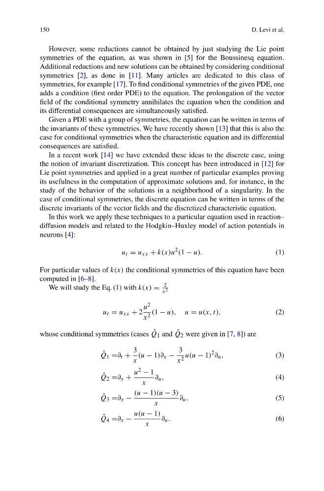
We will study the Eq. (1) with k(x) =
2
x 2
u t = u xx + 2
u 2
x 2 (1 − u), u = u(x, t),
(2)
whose conditional symmetries (cases ˆ
Q 1 and ˆ
Q 2 were given in [7, 8]) are
ˆ
Q 1 =∂ t +
3
x
(u − 1)∂ x −
3
x 2 u(u − 1)
2 ∂ u ,
(3)
ˆ
Q 2 =∂ x +
u 2 − 1
x
∂ u ,
(4)
ˆ
Q 3 =∂ x −
(u − 1)(u − 3)
x
∂ u ,
(5)
ˆ
Q 4 =∂ x −
u(u − 1)
x
∂ u .
(6)
D. Levi et al.
However, some reductions cannot be obtained by just studying the Lie point
symmetries of the equation, as was shown in [5] for the Boussinesq equation.
Additional reductions and new solutions can be obtained by considering conditional
symmetries [2], as done in [11]. Many articles are dedicated to this class of
symmetries, for example [17]. To find conditional symmetries of the given PDE, one
adds a condition (first order PDE) to the equation. The prolongation of the vector
field of the conditional symmetry annihilates the equation when the condition and
its differential consequences are simultaneously satisfied.
Given a PDE with a group of symmetries, the equation can be written in terms of
the invariants of these symmetries. We have recently shown [13] that this is also the
case for conditional symmetries when the characteristic equation and its differential
consequences are satisfied.
In a recent work [14] we have extended these ideas to the discrete case, using
the notion of invariant discretization. This concept has been introduced in [12] for
Lie point symmetries and applied in a great number of particular examples proving
its usefulness in the computation of approximate solutions and, for instance, in the
study of the behavior of the solutions in a neighborhood of a singularity. In the
case of conditional symmetries, the discrete equation can be written in terms of the
discrete invariants of the vector fields and the discretized characteristic equation.
In this work we apply these techniques to a particular equation used in reaction–
diffusion models and related to the Hodgkin–Huxley model of action potentials in
neurons [4]:
u t = u xx + k(x)u
2 (1 − u).
(1)
For particular values of k(x) the conditional symmetries of this equation have been
computed in [6–8].
We will study the Eq. (1) with k(x) =
2
x 2
u t = u xx + 2
u 2
x 2 (1 − u), u = u(x, t),
(2)
whose conditional symmetries (cases ˆ
Q 1 and ˆ
Q 2 were given in [7, 8]) are
ˆ
Q 1 =∂ t +
3
x
(u − 1)∂ x −
3
x 2 u(u − 1)
2 ∂ u ,
(3)
ˆ
Q 2 =∂ x +
u 2 − 1
x
∂ u ,
(4)
ˆ
Q 3 =∂ x −
(u − 1)(u − 3)
x
∂ u ,
(5)
ˆ
Q 4 =∂ x −
u(u − 1)
x
∂ u .
(6)