

Two Dimensional Infrared Spectroscopy …
41
starts with a description of the experimental set-ups of 2D IR spectroscopy. The next
section provides a detailed understanding of the basic principles of the light-matter
interactions and the possible excitation pathways involved. This is followed by the
description of the unique spectral signatures of the different chemical processes in
the 2D IR spectrum. Next, a comprehensive review of various studies in chemistry,
materials and biology using this experimental technique has been put together. This
is followed by a section about the recent technological advances in 2D IR. Finally, we
conclude by stating the future direction and scope of this spectroscopic technique.
2 Experimental Methodology
2D IR spectroscopy involves three light-matter interactions. The commonly used
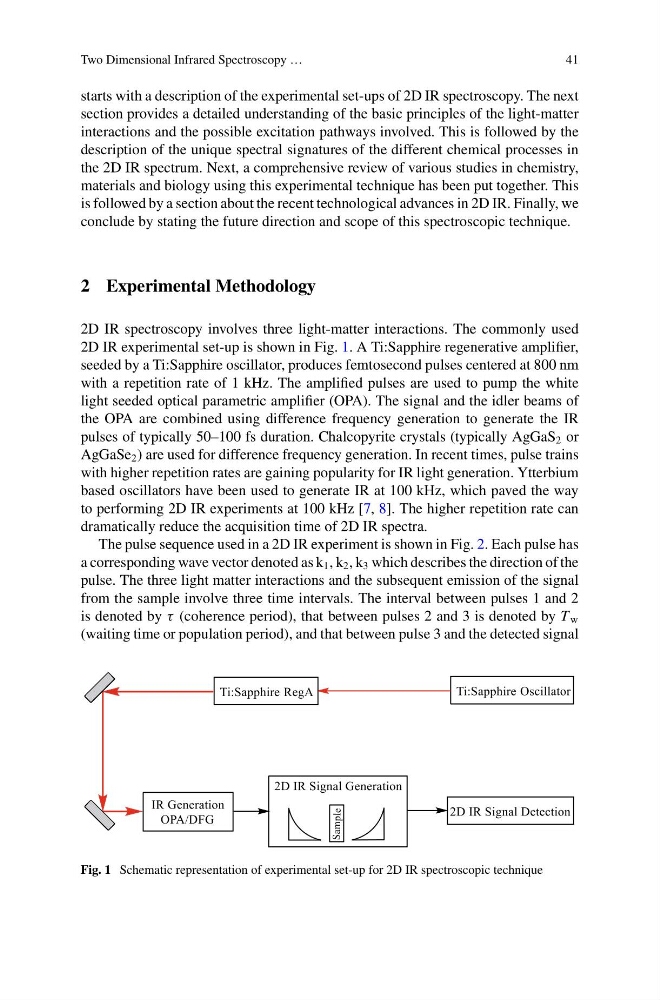
2D IR experimental set-up is shown in Fig. 1. A Ti:Sapphire regenerative amplifier,
seeded by a Ti:Sapphire oscillator, produces femtosecond pulses centered at 800 nm
with a repetition rate of 1 kHz. The amplified pulses are used to pump the white
light seeded optical parametric amplifier (OPA). The signal and the idler beams of
the OPA are combined using difference frequency generation to generate the IR
pulses of typically 50–100 fs duration. Chalcopyrite crystals (typically AgGaS 2 or
AgGaSe 2 ) are used for difference frequency generation. In recent times, pulse trains
with higher repetition rates are gaining popularity for IR light generation. Ytterbium
based oscillators have been used to generate IR at 100 kHz, which paved the way
to performing 2D IR experiments at 100 kHz [7, 8]. The higher repetition rate can
dramatically reduce the acquisition time of 2D IR spectra.
The pulse sequence used in a 2D IR experiment is shown in Fig. 2. Each pulse has
a corresponding wave vector denoted as k 1 , k 2 , k 3 which describes the direction of the
pulse. The three light matter interactions and the subsequent emission of the signal
from the sample involve three time intervals. The interval between pulses 1 and 2
is denoted by τ (coherence period), that between pulses 2 and 3 is denoted by T w
(waiting time or population period), and that between pulse 3 and the detected signal
Fig. 1 Schematic representation of experimental set-up for 2D IR spectroscopic technique
41
starts with a description of the experimental set-ups of 2D IR spectroscopy. The next
section provides a detailed understanding of the basic principles of the light-matter
interactions and the possible excitation pathways involved. This is followed by the
description of the unique spectral signatures of the different chemical processes in
the 2D IR spectrum. Next, a comprehensive review of various studies in chemistry,
materials and biology using this experimental technique has been put together. This
is followed by a section about the recent technological advances in 2D IR. Finally, we
conclude by stating the future direction and scope of this spectroscopic technique.
2 Experimental Methodology
2D IR spectroscopy involves three light-matter interactions. The commonly used
2D IR experimental set-up is shown in Fig. 1. A Ti:Sapphire regenerative amplifier,
seeded by a Ti:Sapphire oscillator, produces femtosecond pulses centered at 800 nm
with a repetition rate of 1 kHz. The amplified pulses are used to pump the white
light seeded optical parametric amplifier (OPA). The signal and the idler beams of
the OPA are combined using difference frequency generation to generate the IR
pulses of typically 50–100 fs duration. Chalcopyrite crystals (typically AgGaS 2 or
AgGaSe 2 ) are used for difference frequency generation. In recent times, pulse trains
with higher repetition rates are gaining popularity for IR light generation. Ytterbium
based oscillators have been used to generate IR at 100 kHz, which paved the way
to performing 2D IR experiments at 100 kHz [7, 8]. The higher repetition rate can
dramatically reduce the acquisition time of 2D IR spectra.
The pulse sequence used in a 2D IR experiment is shown in Fig. 2. Each pulse has
a corresponding wave vector denoted as k 1 , k 2 , k 3 which describes the direction of the
pulse. The three light matter interactions and the subsequent emission of the signal
from the sample involve three time intervals. The interval between pulses 1 and 2
is denoted by τ (coherence period), that between pulses 2 and 3 is denoted by T w
(waiting time or population period), and that between pulse 3 and the detected signal
Fig. 1 Schematic representation of experimental set-up for 2D IR spectroscopic technique