

54
4 Design Optimization of Micromixers
4.4.3 Kriging
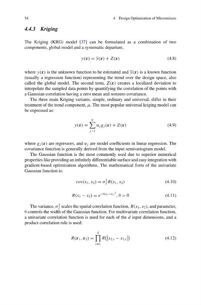
The Kriging (KRG) model [37] can be formulated as a combination of two
components, global model and a systematic departure,
y(x) = y(x) + Z (x)
(4.8)
where y(x) is the unknown function to be estimated and y(x) is a known function
(usually a regression function) representing the trend over the design space, also
called the global model. The second term, Z (x) creates a localized deviation to
interpolate the sampled data points by quantifying the correlation of the points with
a Gaussian correlation having a zero mean and nonzero covariance.
The three main Kriging variants, simple, ordinary and universal, differ in their
treatment of the trend component, μ. The most popular universal kriging model can
be expressed as:
y(x) =
n
j=1
α j g j (x) + Z (x)
(4.9)
where g j (x) are regressors, and α j are model coefficients in linear regression. The
covariance function is generally derived from the input semivariogram model.
The Gaussian function is the most commonly used due to superior numerical
properties like providing an infinitely differentiable surface and easy integration with
gradient-based optimization algorithms. The mathematical form of the univariate
Gaussian function is:
cov(x 1 , x 2 ) = σ
2
f R(x 1 , x 2 )
(4.10)
R(x 1 − x 2 ) = e
−θ|x 1 −x 2 |
2 , θ > 0
(4.11)
The variance, σ
2
f scales the spatial correlation function, R(x 1 , x 2 ), and parameter,
θ controls the width of the Gaussian function. For multivariate correlation function,
a univariate correlation function is used for each of the d input dimensions, and a
product correlation rule is used:
R(x 1 , x 2 ) =
d
i=1
R
x 2,i − x 1,i
(4.12)
4 Design Optimization of Micromixers
4.4.3 Kriging
The Kriging (KRG) model [37] can be formulated as a combination of two
components, global model and a systematic departure,
y(x) = y(x) + Z (x)
(4.8)
where y(x) is the unknown function to be estimated and y(x) is a known function
(usually a regression function) representing the trend over the design space, also
called the global model. The second term, Z (x) creates a localized deviation to
interpolate the sampled data points by quantifying the correlation of the points with
a Gaussian correlation having a zero mean and nonzero covariance.
The three main Kriging variants, simple, ordinary and universal, differ in their
treatment of the trend component, μ. The most popular universal kriging model can
be expressed as:
y(x) =
n
j=1
α j g j (x) + Z (x)
(4.9)
where g j (x) are regressors, and α j are model coefficients in linear regression. The
covariance function is generally derived from the input semivariogram model.
The Gaussian function is the most commonly used due to superior numerical
properties like providing an infinitely differentiable surface and easy integration with
gradient-based optimization algorithms. The mathematical form of the univariate
Gaussian function is:
cov(x 1 , x 2 ) = σ
2
f R(x 1 , x 2 )
(4.10)
R(x 1 − x 2 ) = e
−θ|x 1 −x 2 |
2 , θ > 0
(4.11)
The variance, σ
2
f scales the spatial correlation function, R(x 1 , x 2 ), and parameter,
θ controls the width of the Gaussian function. For multivariate correlation function,
a univariate correlation function is used for each of the d input dimensions, and a
product correlation rule is used:
R(x 1 , x 2 ) =
d
i=1
R
x 2,i − x 1,i
(4.12)