

66
A Structure of Raw Data
A.2 Mechanical Noise Peaks
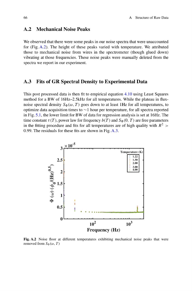
We observed that there were some peaks in our noise spectra that were unaccounted
for (Fig. A.2). The height of these peaks varied with temperature. We attributed
those to mechanical noise from wires in the spectrometer (though glued down)
vibrating at those frequencies. These noise peaks were manually deleted from the
spectra we report in our experiment.
A.3 Fits of GR Spectral Density to Experimental Data
This post processed data is then fit to empirical equation 4.10 using Least Squares
method for a BW of 16Hz–2.5kHz for all temperatures. While the plateau in fluxnoise spectral density S (ω, T ) goes down to at least 1Hz for all temperatures, to
optimize data acquisition times to ∼1 hour per temperature, for all spectra reported
in Fig. 5.1, the lower limit for BW of data for regression analysis is set at 16Hz. The
time constant τ (T ), power law for frequency b(T ) and S (0, T ) are free parameters
in the fitting procedure and fits for all temperatures are of high quality with R 2 >
0.99. The residuals for these fits are shown in Fig. A.3.
10
2
10
3
Frequency (Hz)
0
0.5
1
1.5
2
2.5
3
( ) (
0
/(Hz)
0.5
)
10
-5
1.22
1.50
2.00
3.00
4.00
Temperature (K)
Fig. A.2 Noise floor at different temperatures exhibiting mechanical noise peaks that were
removed from S (ω, T )
A Structure of Raw Data
A.2 Mechanical Noise Peaks
We observed that there were some peaks in our noise spectra that were unaccounted
for (Fig. A.2). The height of these peaks varied with temperature. We attributed
those to mechanical noise from wires in the spectrometer (though glued down)
vibrating at those frequencies. These noise peaks were manually deleted from the
spectra we report in our experiment.
A.3 Fits of GR Spectral Density to Experimental Data
This post processed data is then fit to empirical equation 4.10 using Least Squares
method for a BW of 16Hz–2.5kHz for all temperatures. While the plateau in fluxnoise spectral density S (ω, T ) goes down to at least 1Hz for all temperatures, to
optimize data acquisition times to ∼1 hour per temperature, for all spectra reported
in Fig. 5.1, the lower limit for BW of data for regression analysis is set at 16Hz. The
time constant τ (T ), power law for frequency b(T ) and S (0, T ) are free parameters
in the fitting procedure and fits for all temperatures are of high quality with R 2 >
0.99. The residuals for these fits are shown in Fig. A.3.
10
2
10
3
Frequency (Hz)
0
0.5
1
1.5
2
2.5
3
( ) (
0
/(Hz)
0.5
)
10
-5
1.22
1.50
2.00
3.00
4.00
Temperature (K)
Fig. A.2 Noise floor at different temperatures exhibiting mechanical noise peaks that were
removed from S (ω, T )