

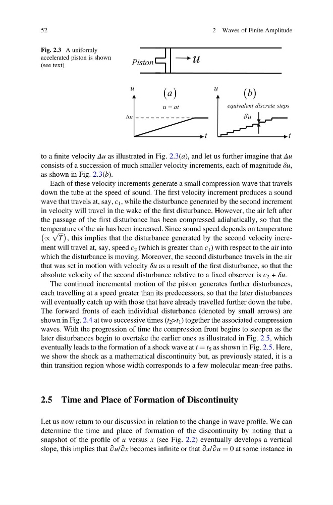
to a finite velocity Δu as illustrated in Fig. 2.3(a), and let us further imagine that Δu
consists of a succession of much smaller velocity increments, each of magnitude δu,
as shown in Fig. 2.3(b).
Each of these velocity increments generate a small compression wave that travels
down the tube at the speed of sound. The first velocity increment produces a sound
wave that travels at, say, c 1 , while the disturbance generated by the second increment
in velocity will travel in the wake of the first disturbance. However, the air left after
the passage of the first disturbance has been compressed adiabatically, so that the
temperature of the air has been increased. Since sound speed depends on temperature
/
ffiffiffi ffi
T
p
À
Á
, this implies that the disturbance generated by the second velocity increment will travel at, say, speed c 2 (which is greater than c 1 ) with respect to the air into
which the disturbance is moving. Moreover, the second disturbance travels in the air
that was set in motion with velocity δu as a result of the first disturbance, so that the
absolute velocity of the second disturbance relative to a fixed observer is c 2 + δu.
The continued incremental motion of the piston generates further disturbances,
each travelling at a speed greater than its predecessors, so that the later disturbances
will eventually catch up with those that have already travelled further down the tube.
The forward fronts of each individual disturbance (denoted by small arrows) are
shown in Fig. 2.4 at two successive times (t 2 >t 1 ) together the associated compression
waves. With the progression of time the compression front begins to steepen as the
later disturbances begin to overtake the earlier ones as illustrated in Fig. 2.5, which
eventually leads to the formation of a shock wave at t ¼ t 5 as shown in Fig. 2.5. Here,
we show the shock as a mathematical discontinuity but, as previously stated, it is a
thin transition region whose width corresponds to a few molecular mean-free paths.
2.5 Time and Place of Formation of Discontinuity
Let us now return to our discussion in relation to the change in wave profile. We can
determine the time and place of formation of the discontinuity by noting that a
snapshot of the profile of u versus x (see Fig. 2.2) eventually develops a vertical
slope, this implies that ∂u/∂x becomes infinite or that ∂x/∂u ¼ 0 at some instance in
Fig. 2.3 A uniformly
accelerated piston is shown
(see text)
52
2 Waves of Finite Amplitude
consists of a succession of much smaller velocity increments, each of magnitude δu,
as shown in Fig. 2.3(b).
Each of these velocity increments generate a small compression wave that travels
down the tube at the speed of sound. The first velocity increment produces a sound
wave that travels at, say, c 1 , while the disturbance generated by the second increment
in velocity will travel in the wake of the first disturbance. However, the air left after
the passage of the first disturbance has been compressed adiabatically, so that the
temperature of the air has been increased. Since sound speed depends on temperature
/
ffiffiffi ffi
T
p
À
Á
, this implies that the disturbance generated by the second velocity increment will travel at, say, speed c 2 (which is greater than c 1 ) with respect to the air into
which the disturbance is moving. Moreover, the second disturbance travels in the air
that was set in motion with velocity δu as a result of the first disturbance, so that the
absolute velocity of the second disturbance relative to a fixed observer is c 2 + δu.
The continued incremental motion of the piston generates further disturbances,
each travelling at a speed greater than its predecessors, so that the later disturbances
will eventually catch up with those that have already travelled further down the tube.
The forward fronts of each individual disturbance (denoted by small arrows) are
shown in Fig. 2.4 at two successive times (t 2 >t 1 ) together the associated compression
waves. With the progression of time the compression front begins to steepen as the
later disturbances begin to overtake the earlier ones as illustrated in Fig. 2.5, which
eventually leads to the formation of a shock wave at t ¼ t 5 as shown in Fig. 2.5. Here,
we show the shock as a mathematical discontinuity but, as previously stated, it is a
thin transition region whose width corresponds to a few molecular mean-free paths.
2.5 Time and Place of Formation of Discontinuity
Let us now return to our discussion in relation to the change in wave profile. We can
determine the time and place of formation of the discontinuity by noting that a
snapshot of the profile of u versus x (see Fig. 2.2) eventually develops a vertical
slope, this implies that ∂u/∂x becomes infinite or that ∂x/∂u ¼ 0 at some instance in
Fig. 2.3 A uniformly
accelerated piston is shown
(see text)
52
2 Waves of Finite Amplitude