

Appendix B
Some Numerical Results for a Closed Shock Tube
In this appendix we will consider the shock tube with the same initial conditions that
was discussed in Sect. 4.8.7 but in this particular case we will assume that the tube is
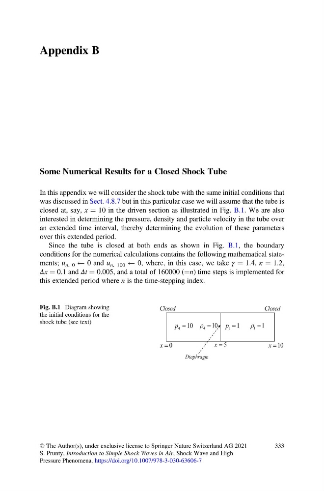
closed at, say, x ¼ 10 in the driven section as illustrated in Fig. B.1. We are also
interested in determining the pressure, density and particle velocity in the tube over
an extended time interval, thereby determining the evolution of these parameters
over this extended period.
Since the tube is closed at both ends as shown in Fig. B.1, the boundary
conditions for the numerical calculations contains the following mathematical statements; u n, 0
0 and u n, 100
0, where, in this case, we take γ ¼ 1.4, κ ¼ 1.2,
Δx ¼ 0.1 and Δt ¼ 0.005, and a total of 160000 (¼n) time steps is implemented for
this extended period where n is the time-stepping index.
Fig. B.1 Diagram showing
the initial conditions for the
shock tube (see text)
© The Author(s), under exclusive license to Springer Nature Switzerland AG 2021
S. Prunty, Introduction to Simple Shock Waves in Air, Shock Wave and High
Pressure Phenomena, https://doi.org/10.1007/978-3-030-63606-7
333
Some Numerical Results for a Closed Shock Tube
In this appendix we will consider the shock tube with the same initial conditions that
was discussed in Sect. 4.8.7 but in this particular case we will assume that the tube is
closed at, say, x ¼ 10 in the driven section as illustrated in Fig. B.1. We are also
interested in determining the pressure, density and particle velocity in the tube over
an extended time interval, thereby determining the evolution of these parameters
over this extended period.
Since the tube is closed at both ends as shown in Fig. B.1, the boundary
conditions for the numerical calculations contains the following mathematical statements; u n, 0
0 and u n, 100
0, where, in this case, we take γ ¼ 1.4, κ ¼ 1.2,
Δx ¼ 0.1 and Δt ¼ 0.005, and a total of 160000 (¼n) time steps is implemented for
this extended period where n is the time-stepping index.
Fig. B.1 Diagram showing
the initial conditions for the
shock tube (see text)
© The Author(s), under exclusive license to Springer Nature Switzerland AG 2021
S. Prunty, Introduction to Simple Shock Waves in Air, Shock Wave and High
Pressure Phenomena, https://doi.org/10.1007/978-3-030-63606-7
333