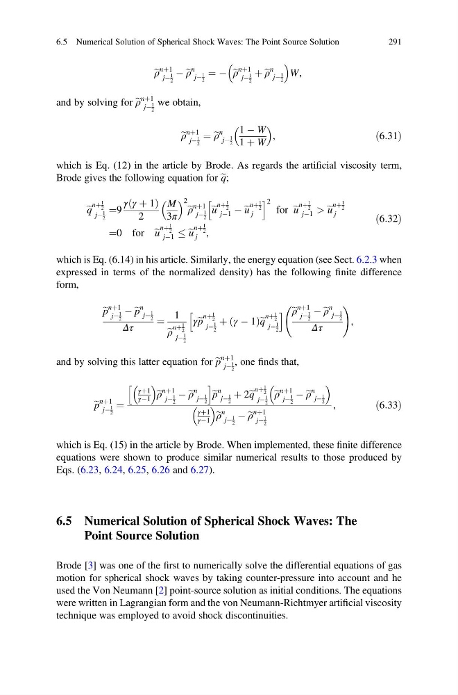
e ρ
nþ1
jÀ
1
2
À e ρ
n
jÀ
1
2
¼ À e ρ
nþ1
jÀ
1
2
þ e ρ
n
jÀ
1
2
W,
and by solving for e ρ
nþ1
jÀ
1
2
we obtain,
e ρ
nþ1
jÀ
1
2
¼ e ρ
n
jÀ
1
2
1 À W
1 þ W
,
ð6:31Þ
which is Eq. (12) in the article by Brode. As regards the artificial viscosity term,
Brode gives the following equation for e q;
e q
nþ
1
2
jÀ
1
2
¼9
γ γ þ 1
ð
Þ
2
M
3π
2
e ρ
nþ1
jÀ
1
2
e u
nþ
1
2
jÀ1 À e u
nþ
1
2
j
h
i 2
for e u
nþ
1
2
jÀ1 > e u
nþ
1
2
j
¼0 for e u
nþ
1
2
jÀ1
e u
nþ
1
2
j ,
ð6:32Þ
which is Eq. (6.14) in his article. Similarly, the energy equation (see Sect. 6.2.3 when
expressed in terms of the normalized density) has the following finite difference
form,
e p
nþ1
jÀ
1
2
À e p
n
jÀ
1
2
Δτ
¼
1
e ρ
nþ
1
2
jÀ
1
2
γe p
nþ
1
2
jÀ
1
2
þ γ À 1
ð
Þe q
nþ
1
2
jÀ
1
2
h
i e ρ
nþ1
jÀ
1
2
À e ρ
n
jÀ
1
2
Δτ
!
,
and by solving this latter equation for e p
nþ1
jÀ
1
2
, one finds that,
e p
nþ1
jÀ
1
2
¼
γþ1
γÀ1
e ρ
nþ1
jÀ
1
2
À e ρ
n
jÀ
1
2
h
i
e p
n
jÀ
1
2
þ 2e q
nþ
1
2
jÀ
1
2
e ρ
nþ1
jÀ
1
2
À e ρ
n
jÀ
1
2
γþ1
γÀ1
e ρ
n
jÀ
1
2
À e ρ
nþ1
jÀ
1
2
,
ð6:33Þ
which is Eq. (15) in the article by Brode. When implemented, these finite difference
equations were shown to produce similar numerical results to those produced by
Eqs. (6.23, 6.24, 6.25, 6.26 and 6.27).
6.5 Numerical Solution of Spherical Shock Waves: The
Point Source Solution
Brode [3] was one of the first to numerically solve the differential equations of gas
motion for spherical shock waves by taking counter-pressure into account and he
used the Von Neumann [2] point-source solution as initial conditions. The equations
were written in Lagrangian form and the von Neumann-Richtmyer artificial viscosity
technique was employed to avoid shock discontinuities.
6.5 Numerical Solution of Spherical Shock Waves: The Point Source Solution
291