6.3 Conservation Equations in Spherical Geometry: A
Summary
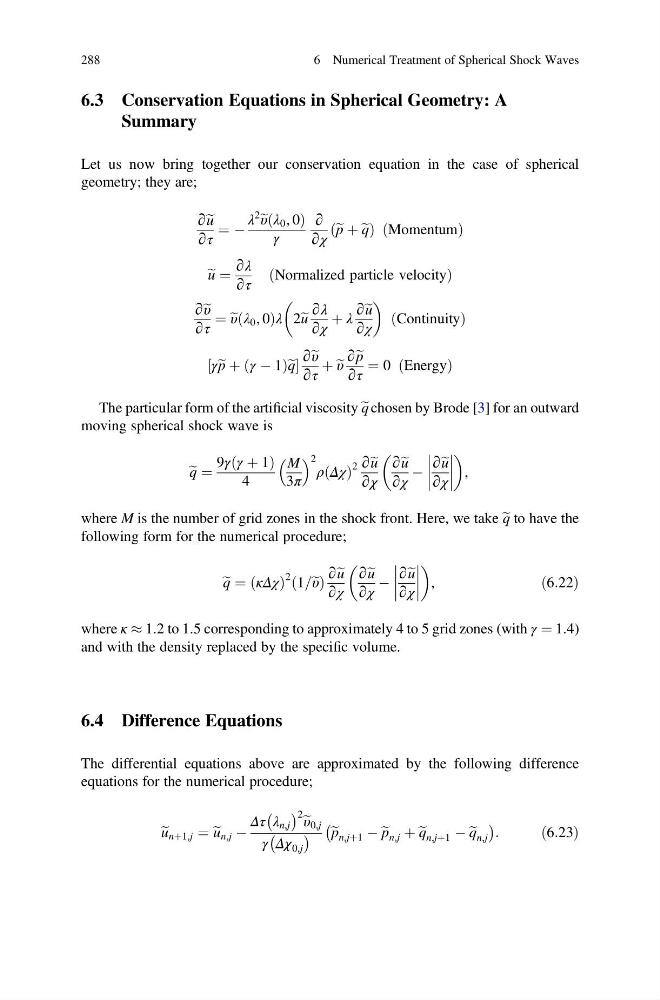
Let us now bring together our conservation equation in the case of spherical
geometry; they are;
∂e u
∂τ
¼ À
λ
2
e υ λ 0 , 0
ð
Þ
γ
∂
∂χ
e p þ e q
ð
Þ Momentum
ð
Þ
e u ¼
∂λ
∂τ
Normalized particle velocity
ð
Þ
∂e υ
∂τ
¼ e υ λ 0 , 0
ð
Þλ 2e u
∂λ
∂χ
þ λ
∂e u
∂χ
Continuity
ð
Þ
γe p þ γ À 1
ð
Þe q
½
Š
∂e υ
∂τ
þ e υ
∂e p
∂τ
¼ 0 Energy
ð
Þ
The particular form of the artificial viscosity e q chosen by Brode [3] for an outward
moving spherical shock wave is
e q ¼
9γ γ þ 1
ð
Þ
4
M
3π
2
ρ Δχ
ð Þ
2 ∂e u
∂χ
∂e u
∂χ
À
∂e u
∂χ
,
where M is the number of grid zones in the shock front. Here, we take e q to have the
following form for the numerical procedure;
e q ¼ κΔχ
ð
Þ
2 1=e υ
ð Þ
∂e u
∂χ
∂e u
∂χ
À
∂e u
∂χ
,
ð6:22Þ
where κ % 1.2 to 1.5 corresponding to approximately 4 to 5 grid zones (with γ ¼ 1.4)
and with the density replaced by the specific volume.
6.4 Difference Equations
The differential equations above are approximated by the following difference
equations for the numerical procedure;
e u nþ1,j ¼ e u n,j À
Δτ λ n,j
À Á 2 e υ 0,j
γ Δχ 0,j
À
Á e p n,jþ1 À e p n,j þ e q n,jþ1 À e q n,j
À
Á :
ð6:23Þ
288
6 Numerical Treatment of Spherical Shock Waves