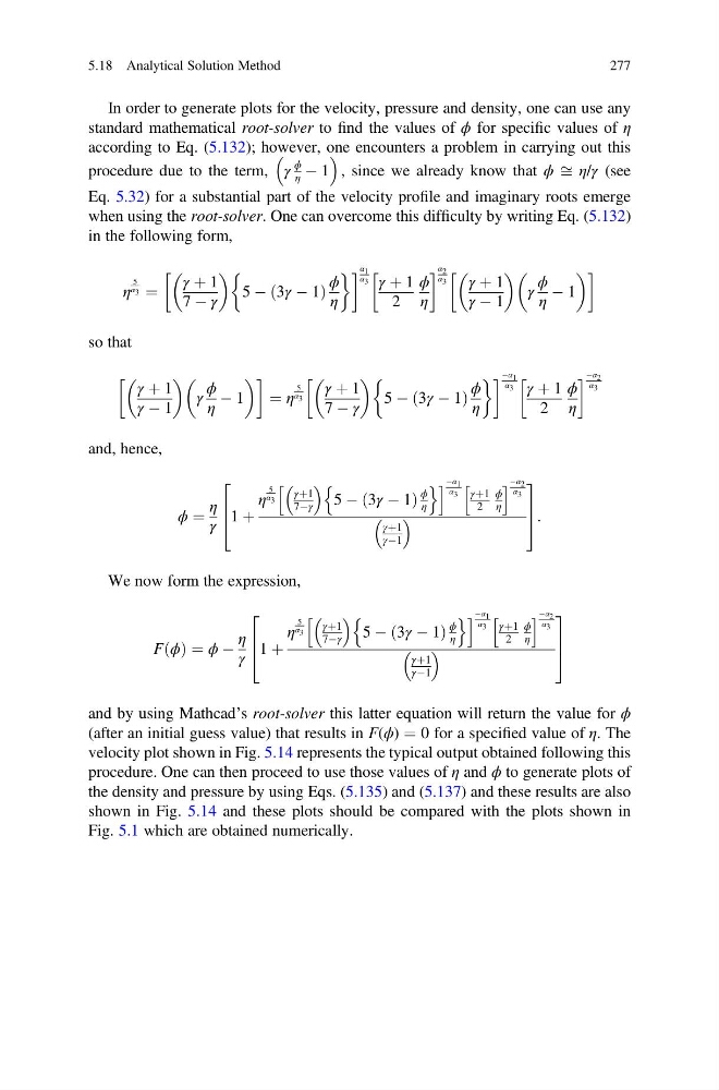
In order to generate plots for the velocity, pressure and density, one can use any
standard mathematical root-solver to find the values of ϕ for specific values of η
according to Eq. (5.132); however, one encounters a problem in carrying out this
procedure due to the term, γ
ϕ
η À 1
, since we already know that ϕ ffi η/γ (see
Eq. 5.32) for a substantial part of the velocity profile and imaginary roots emerge
when using the root-solver. One can overcome this difficulty by writing Eq. (5.132)
in the following form,
η
5
α 3 ¼
γ þ 1
7 À γ
5 À 3γ À 1
ð
Þ
ϕ
η
&
' ! α 1
α 3 γ þ 1
2
ϕ
η
! α 2
α 3
γ þ 1
γ À 1
γ
ϕ
η
À 1
!
so that
γ þ 1
γ À 1
γ
ϕ
η
À 1
!
¼ η
5
α 3
γ þ 1
7 À γ
5 À 3γ À 1
ð
Þ
ϕ
η
&
' ! Àα 1
α 3
γ þ 1
2
ϕ
η
! Àα 2
α 3
and, hence,
ϕ ¼
η
γ
1 þ
η
5
α 3
γþ1
7Àγ
5 À 3γ À 1
ð
Þ
ϕ
η
n
o
h
i Àα 1
α 3
γþ1
2
ϕ
η
h
i Àα 2
α 3
γþ1
γÀ1
2
6
4
3
7
5:
We now form the expression,
F ϕ
ð Þ ¼ ϕ À
η
γ
1 þ
η
5
α 3
γþ1
7Àγ
5 À 3γ À 1
ð
Þ
ϕ
η
n
o
h
i Àα 1
α 3
γþ1
2
ϕ
η
h
i Àα 2
α 3
γþ1
γÀ1
2
6
4
3
7
5
and by using Mathcad’s root-solver this latter equation will return the value for ϕ
(after an initial guess value) that results in F(ϕ) ¼ 0 for a specified value of η. The
velocity plot shown in Fig. 5.14 represents the typical output obtained following this
procedure. One can then proceed to use those values of η and ϕ to generate plots of
the density and pressure by using Eqs. (5.135) and (5.137) and these results are also
shown in Fig. 5.14 and these plots should be compared with the plots shown in
Fig. 5.1 which are obtained numerically.
5.18 Analytical Solution Method
277