

ϕ η
ð Þ ¼ η=γ,
ð5:32Þ
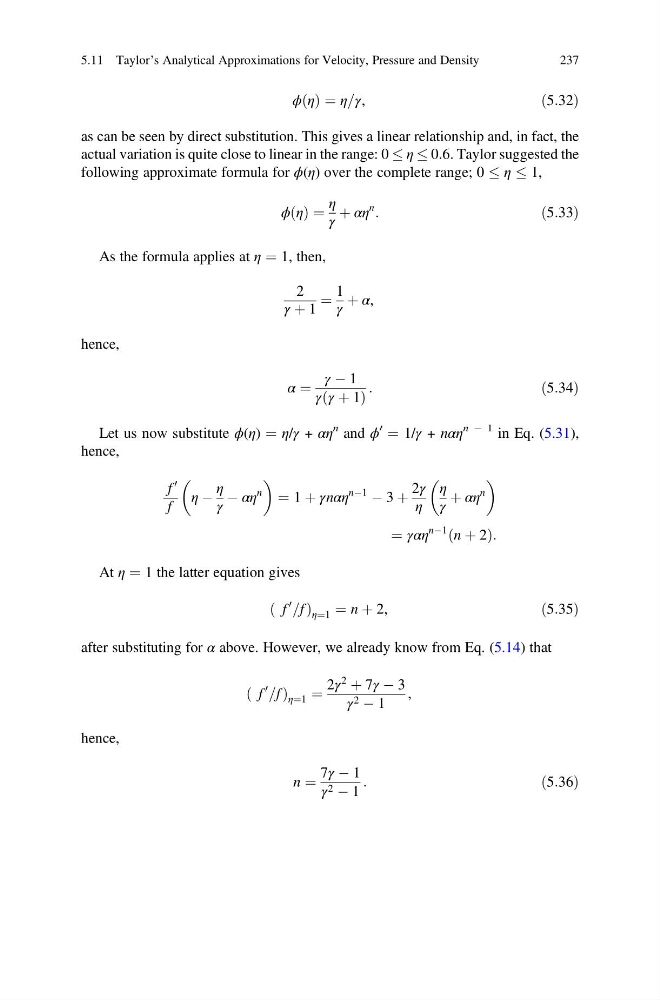
as can be seen by direct substitution. This gives a linear relationship and, in fact, the
actual variation is quite close to linear in the range: 0 η 0.6. Taylor suggested the
following approximate formula for ϕ(η) over the complete range; 0 η 1,
ϕ η
ð Þ ¼
η
γ
þ αη
n
:
ð5:33Þ
As the formula applies at η ¼ 1, then,
2
γ þ 1
¼
1
γ
þ α,
hence,
α ¼
γ À 1
γ γ þ 1
ð
Þ
:
ð5:34Þ
Let us now substitute ϕ(η) ¼ η/γ + αη
n and ϕ
0
¼ 1/γ + nαη
n À 1 in Eq. (5.31),
hence,
f
0
f
η À
η
γ
À αη
n
¼ 1 þ γnαη
nÀ1
À 3 þ
2γ
η
η
γ
þ αη
n
¼ γαη
nÀ1 n þ 2
ð
Þ:
At η ¼ 1 the latter equation gives
f
0
=f
ð
Þ η¼1 ¼ n þ 2,
ð5:35Þ
after substituting for α above. However, we already know from Eq. (5.14) that
f
0
=f
ð
Þ η¼1 ¼
2γ
2
þ 7γ À 3
γ 2 À 1
,
hence,
n ¼
7γ À 1
γ 2 À 1
:
ð5:36Þ
5.11 Taylor’s Analytical Approximations for Velocity, Pressure and Density
237
ð Þ ¼ η=γ,
ð5:32Þ
as can be seen by direct substitution. This gives a linear relationship and, in fact, the
actual variation is quite close to linear in the range: 0 η 0.6. Taylor suggested the
following approximate formula for ϕ(η) over the complete range; 0 η 1,
ϕ η
ð Þ ¼
η
γ
þ αη
n
:
ð5:33Þ
As the formula applies at η ¼ 1, then,
2
γ þ 1
¼
1
γ
þ α,
hence,
α ¼
γ À 1
γ γ þ 1
ð
Þ
:
ð5:34Þ
Let us now substitute ϕ(η) ¼ η/γ + αη
n and ϕ
0
¼ 1/γ + nαη
n À 1 in Eq. (5.31),
hence,
f
0
f
η À
η
γ
À αη
n
¼ 1 þ γnαη
nÀ1
À 3 þ
2γ
η
η
γ
þ αη
n
¼ γαη
nÀ1 n þ 2
ð
Þ:
At η ¼ 1 the latter equation gives
f
0
=f
ð
Þ η¼1 ¼ n þ 2,
ð5:35Þ
after substituting for α above. However, we already know from Eq. (5.14) that
f
0
=f
ð
Þ η¼1 ¼
2γ
2
þ 7γ À 3
γ 2 À 1
,
hence,
n ¼
7γ À 1
γ 2 À 1
:
ð5:36Þ
5.11 Taylor’s Analytical Approximations for Velocity, Pressure and Density
237