

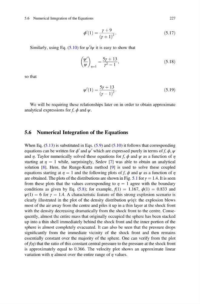
ϕ
0 1
ð Þ ¼
γ þ 9
γ þ 1
ð
Þ
2
:
ð5:17Þ
Similarly, using Eq. (5.10) for ψ
0 /ψ it is easy to show that
ψ
0
ψ
η¼1
¼
5γ þ 13
γ 2 À 1
,
ð5:18Þ
so that
ψ
0 1
ð Þ ¼
5γ þ 13
γ À 1
ð
Þ
2
:
ð5:19Þ
We will be requiring these relationships later on in order to obtain approximate
analytical expressions for f, ϕ and ψ.
5.6 Numerical Integration of the Equations
When Eq. (5.13) is substituted in Eqs. (5.9) and (5.10) it follows that corresponding
equations can be written for ϕ
0 and ψ
0 which are expressed purely in terms of f, ϕ, ψ
and η. Taylor numerically solved these equations for f, ϕ and ψ as a function of η
starting at η ¼ 1 while, surprisingly, Sedov [7] was able to obtain an analytical
solution [8]. Here, the Runge-Kutta method [9] is used to solve these coupled
equations starting at η ¼ 1 and the following plots of f, ϕ and ψ as a function of η
are obtained. The plots of the distributions are shown in Fig. 5.1 for γ ¼ 1.4. It is seen
from these plots that the values corresponding to η ¼ 1 agree with the boundary
conditions as given by Eq. (5.8); for example, f(1) ¼ 1.167, ϕ(1) ¼ 0.833 and
ψ(1) ¼ 6 for γ ¼ 1.4. A characteristic feature of this strong explosion scenario is
clearly illustrated in the plot of the density distribution ψ(η): the explosion blows
most of the air away from the centre and piles it up in a thin layer at the shock front
with the density decreasing dramatically from the shock front to the centre. Consequently, almost the entire mass that originally occupied the sphere has been stacked
up into a thin shell immediately behind the shock front and the inner portion of the
sphere is almost completely evacuated. It can also be seen that the pressure drops
significantly from the immediate vicinity of the shock front and then remains
essentially constant over the majority of the sphere. One can verify from the plot
of f(η) that the ratio of this constant central pressure to the pressure at the shock front
is approximately equal to 0.366. The velocity plot shows an approximate linear
variation with η almost over the entire range of η values.
5.6 Numerical Integration of the Equations
227
0 1
ð Þ ¼
γ þ 9
γ þ 1
ð
Þ
2
:
ð5:17Þ
Similarly, using Eq. (5.10) for ψ
0 /ψ it is easy to show that
ψ
0
ψ
η¼1
¼
5γ þ 13
γ 2 À 1
,
ð5:18Þ
so that
ψ
0 1
ð Þ ¼
5γ þ 13
γ À 1
ð
Þ
2
:
ð5:19Þ
We will be requiring these relationships later on in order to obtain approximate
analytical expressions for f, ϕ and ψ.
5.6 Numerical Integration of the Equations
When Eq. (5.13) is substituted in Eqs. (5.9) and (5.10) it follows that corresponding
equations can be written for ϕ
0 and ψ
0 which are expressed purely in terms of f, ϕ, ψ
and η. Taylor numerically solved these equations for f, ϕ and ψ as a function of η
starting at η ¼ 1 while, surprisingly, Sedov [7] was able to obtain an analytical
solution [8]. Here, the Runge-Kutta method [9] is used to solve these coupled
equations starting at η ¼ 1 and the following plots of f, ϕ and ψ as a function of η
are obtained. The plots of the distributions are shown in Fig. 5.1 for γ ¼ 1.4. It is seen
from these plots that the values corresponding to η ¼ 1 agree with the boundary
conditions as given by Eq. (5.8); for example, f(1) ¼ 1.167, ϕ(1) ¼ 0.833 and
ψ(1) ¼ 6 for γ ¼ 1.4. A characteristic feature of this strong explosion scenario is
clearly illustrated in the plot of the density distribution ψ(η): the explosion blows
most of the air away from the centre and piles it up in a thin layer at the shock front
with the density decreasing dramatically from the shock front to the centre. Consequently, almost the entire mass that originally occupied the sphere has been stacked
up into a thin shell immediately behind the shock front and the inner portion of the
sphere is almost completely evacuated. It can also be seen that the pressure drops
significantly from the immediate vicinity of the shock front and then remains
essentially constant over the majority of the sphere. One can verify from the plot
of f(η) that the ratio of this constant central pressure to the pressure at the shock front
is approximately equal to 0.366. The velocity plot shows an approximate linear
variation with η almost over the entire range of η values.
5.6 Numerical Integration of the Equations
227