

where n is the time-stepping index and the numerical output for the piston’s velocity
and position as a function of time t (¼nΔt) is shown in Fig. 4.67 where Δt ¼ 0.04. It
is assumed that the ambient pressure and density have unity values. The short
duration (0 n 500) piston motion generates the outgoing shock whose pressure
as a function of position is shown plotted in Fig. 4.68 at t ¼ 2000Δt and at
t ¼ 2600Δt. Its reflection from an end wall located at x ¼ 160 is shown in the
same figure at t ¼ 3100Δt and at t ¼ 3300Δt. For t > 3000Δt one observes the second
outward moving shock wave on its collision course with the reflected shock. Based
on our discussion in Sect. 4.8.9 we note that this reflected shock propagates with
decreasing intensity and Fig. 4.69 shows the further advancement of these shocks
prior to collision.
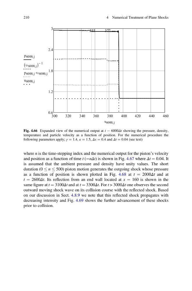
Fig. 4.66 Expanded view of the numerical output at t ¼ 6000Δt showing the pressure, density,
temperature and particle velocity as a function of position. For the numerical procedure the
following parameters apply; γ ¼ 1.4, κ ¼ 1.5, Δx ¼ 0.4 and Δt ¼ 0.04 (see text)
210
4 Numerical Treatment of Plane Shocks
and position as a function of time t (¼nΔt) is shown in Fig. 4.67 where Δt ¼ 0.04. It
is assumed that the ambient pressure and density have unity values. The short
duration (0 n 500) piston motion generates the outgoing shock whose pressure
as a function of position is shown plotted in Fig. 4.68 at t ¼ 2000Δt and at
t ¼ 2600Δt. Its reflection from an end wall located at x ¼ 160 is shown in the
same figure at t ¼ 3100Δt and at t ¼ 3300Δt. For t > 3000Δt one observes the second
outward moving shock wave on its collision course with the reflected shock. Based
on our discussion in Sect. 4.8.9 we note that this reflected shock propagates with
decreasing intensity and Fig. 4.69 shows the further advancement of these shocks
prior to collision.
Fig. 4.66 Expanded view of the numerical output at t ¼ 6000Δt showing the pressure, density,
temperature and particle velocity as a function of position. For the numerical procedure the
following parameters apply; γ ¼ 1.4, κ ¼ 1.5, Δx ¼ 0.4 and Δt ¼ 0.04 (see text)
210
4 Numerical Treatment of Plane Shocks