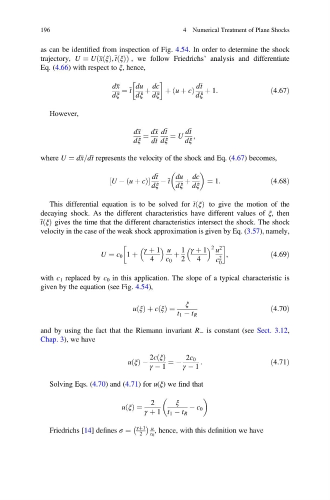
as can be identified from inspection of Fig. 4.54. In order to determine the shock
trajectory, U U x ξ
ð Þ, t ξ
ð Þ
ð
Þ, we follow Friedrichs’ analysis and differentiate
Eq. (4.66) with respect to ξ, hence,
dx
dξ
¼ t
du
dξ
þ
dc
dξ
!
þ u þ c
ð
Þ
dt
dξ
þ 1:
ð4:67Þ
However,
dx
dξ
¼
dx
dt
dt
dξ
¼ U
dt
dξ
,
where U ¼ dx=dt represents the velocity of the shock and Eq. (4.67) becomes,
U À u þ c
ð
Þ
½
Š
dt
dξ
À t
du
dξ
þ
dc
dξ
¼ 1:
ð4:68Þ
This differential equation is to be solved for t ξ
ð Þ to give the motion of the
decaying shock. As the different characteristics have different values of ξ, then
t ξ
ð Þ gives the time that the different characteristics intersect the shock. The shock
velocity in the case of the weak shock approximation is given by Eq. (3.57), namely,
U ¼ c 0 1 þ
γ þ 1
4
u
c 0
þ
1
2
γ þ 1
4
2 u
2
c 2
0
!
,
ð4:69Þ
with c 1 replaced by c 0 in this application. The slope of a typical characteristic is
given by the equation (see Fig. 4.54),
u ξ
ð Þ þ c ξ
ð Þ ¼
ξ
t 1 À t R
ð4:70Þ
and by using the fact that the Riemann invariant R À is constant (see Sect. 3.12,
Chap. 3), we have
u ξ
ð Þ À
2c ξ
ð Þ
γ À 1
¼ À
2c 0
γ À 1
:
ð4:71Þ
Solving Eqs. (4.70) and (4.71) for u(ξ) we find that
u ξ
ð Þ ¼
2
γ þ 1
ξ
t 1 À t R
À c 0
Friedrichs [14] defines σ ¼
γþ1
2
À Á u
c 0
, hence, with this definition we have
196
4 Numerical Treatment of Plane Shocks