

is not known in advance but, instead, is governed by the differential equations
themselves. In reality, however, when the effects of viscosity and thermal conduction are included in the momentum and energy equations the shock wave is no longer
a discontinuous front, but a very steep continuous transition region whose length is a
few molecular mean free paths as previously noted. Accordingly, the spatial grid size
in the finite difference equations would need to be much smaller than the molecular
mean free path in order to realistically model the shock transition region. This aspect
will be referred to at a later stage.
In order to deal with shocks Von Neumann and Richtmyer [1] introduced a
technique that avoids the need for any boundary conditions referred to above and
treats the calculation as if there were no shocks present at all. Instead, the shocks
appear as near-discontinuities that move through the fluid with essentially the correct
speed and across which the thermodynamic variables approximate the predictions of
the Rankine-Hugoniot relations. The method proposed by Von Neumann and
Richtmyer introduces a dissipative mechanism in the form of an artificial viscosity
into the equations so that the shocks are replaced by a thin layer where the pressure,
density, temperature and velocity vary rapidly but continuously and it means that the
shock acquires a thickness somewhat greater than the spacing of the points used in
the numerical procedure. Consequently, the difficult problem of applying boundary
conditions at the shock is avoided. The form of the artificial viscosity introduced by
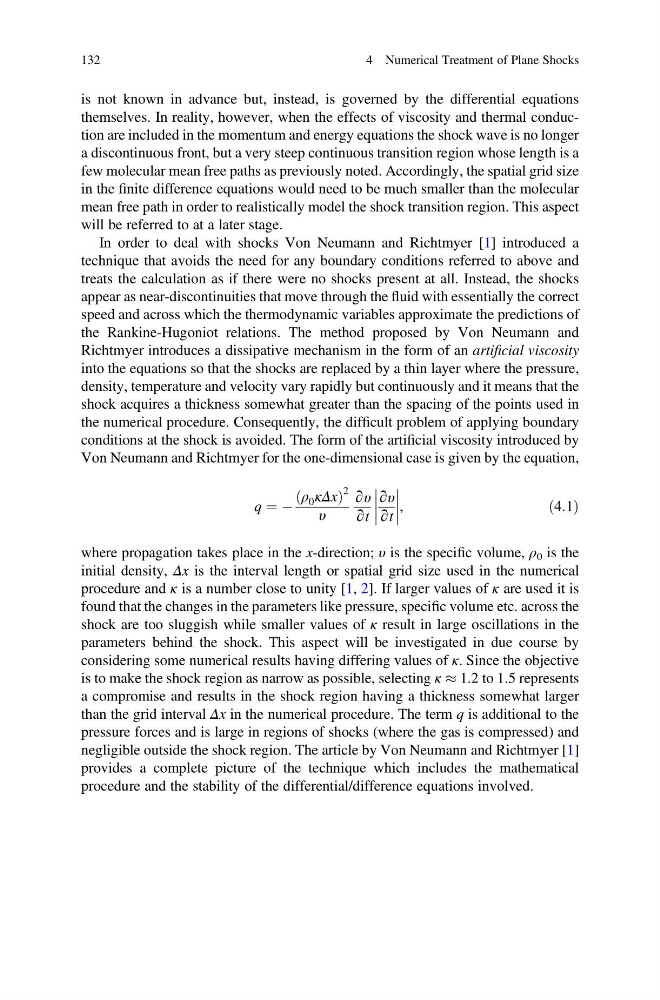
Von Neumann and Richtmyer for the one-dimensional case is given by the equation,
q ¼ À
ρ 0 κΔx
ð
Þ
2
υ
∂υ
∂t
∂υ
∂t
,
ð4:1Þ
where propagation takes place in the x-direction; υ is the specific volume, ρ 0 is the
initial density, Δx is the interval length or spatial grid size used in the numerical
procedure and κ is a number close to unity [1, 2]. If larger values of κ are used it is
found that the changes in the parameters like pressure, specific volume etc. across the
shock are too sluggish while smaller values of κ result in large oscillations in the
parameters behind the shock. This aspect will be investigated in due course by
considering some numerical results having differing values of κ. Since the objective
is to make the shock region as narrow as possible, selecting κ % 1.2 to 1.5 represents
a compromise and results in the shock region having a thickness somewhat larger
than the grid interval Δx in the numerical procedure. The term q is additional to the
pressure forces and is large in regions of shocks (where the gas is compressed) and
negligible outside the shock region. The article by Von Neumann and Richtmyer [1]
provides a complete picture of the technique which includes the mathematical
procedure and the stability of the differential/difference equations involved.
132
4 Numerical Treatment of Plane Shocks
themselves. In reality, however, when the effects of viscosity and thermal conduction are included in the momentum and energy equations the shock wave is no longer
a discontinuous front, but a very steep continuous transition region whose length is a
few molecular mean free paths as previously noted. Accordingly, the spatial grid size
in the finite difference equations would need to be much smaller than the molecular
mean free path in order to realistically model the shock transition region. This aspect
will be referred to at a later stage.
In order to deal with shocks Von Neumann and Richtmyer [1] introduced a
technique that avoids the need for any boundary conditions referred to above and
treats the calculation as if there were no shocks present at all. Instead, the shocks
appear as near-discontinuities that move through the fluid with essentially the correct
speed and across which the thermodynamic variables approximate the predictions of
the Rankine-Hugoniot relations. The method proposed by Von Neumann and
Richtmyer introduces a dissipative mechanism in the form of an artificial viscosity
into the equations so that the shocks are replaced by a thin layer where the pressure,
density, temperature and velocity vary rapidly but continuously and it means that the
shock acquires a thickness somewhat greater than the spacing of the points used in
the numerical procedure. Consequently, the difficult problem of applying boundary
conditions at the shock is avoided. The form of the artificial viscosity introduced by
Von Neumann and Richtmyer for the one-dimensional case is given by the equation,
q ¼ À
ρ 0 κΔx
ð
Þ
2
υ
∂υ
∂t
∂υ
∂t
,
ð4:1Þ
where propagation takes place in the x-direction; υ is the specific volume, ρ 0 is the
initial density, Δx is the interval length or spatial grid size used in the numerical
procedure and κ is a number close to unity [1, 2]. If larger values of κ are used it is
found that the changes in the parameters like pressure, specific volume etc. across the
shock are too sluggish while smaller values of κ result in large oscillations in the
parameters behind the shock. This aspect will be investigated in due course by
considering some numerical results having differing values of κ. Since the objective
is to make the shock region as narrow as possible, selecting κ % 1.2 to 1.5 represents
a compromise and results in the shock region having a thickness somewhat larger
than the grid interval Δx in the numerical procedure. The term q is additional to the
pressure forces and is large in regions of shocks (where the gas is compressed) and
negligible outside the shock region. The article by Von Neumann and Richtmyer [1]
provides a complete picture of the technique which includes the mathematical
procedure and the stability of the differential/difference equations involved.
132
4 Numerical Treatment of Plane Shocks