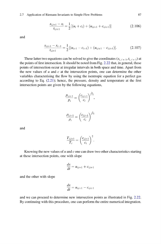
x i,iþ1 À x i
t i,iþ1
¼
1
2
u i þ c i
ð
Þþ u i,iþ1 þ c i,iþ1
ð
Þ
½
Š
ð 2:106Þ
and
x i,iþ1 À x iþ1
t i,iþ1
¼
1
2
u iþ1 À c iþ1
ð
Þþ u i,iþ1 À c i,iþ1
ð
Þ
½
Š :
ð2:107Þ
These latter two equations can be solved to give the coordinates (x i, i + 1 , t i, i + 1 ) at
the points of first intersection. It should be noted from Fig. 2.22 that, in general, these
points of intersection occur at irregular intervals in both space and time. Apart from
the new values of u and c at the intersection points, one can determine the other
variables characterising the flow by using the isentropic equation for a perfect gas
according to Eq. (2.21); hence, the pressure, density and temperature at the first
intersection points are given by the following equations,
p i,iþ1
p i
¼
c i,iþ1
c i
2γ
γÀ1
,
ρ i,iþ1
ρ i
¼
c i,iþ1
c i
2
γÀ1
and
T i,iþ1
T i
¼
c i,iþ1
c i
2
:
Knowing the new values of u and c one can draw two other characteristics starting
at these intersection points, one with slope
dx
dt
¼ u i,iþ1 þ c i,iþ1
and the other with slope
dx
dt
¼ u i,iþ1 À c i,iþ1
and we can proceed to determine new intersection points as illustrated in Fig. 2.22.
By continuing with this procedure, one can perform the entire numerical integration.
2.7 Application of Riemann Invariants to Simple Flow Problems
87