

Elements of Modern Physics
72
dynamical observables that their average values must be real. It is easy show
from Eq. (3.30) that both r and p have real average values and are acceptable
as dynamical observables. On the other hand, xp x is not an observable though
the angular momentum r × p can be shown to have a real average value and
hence is acceptable as a dynamical observable.
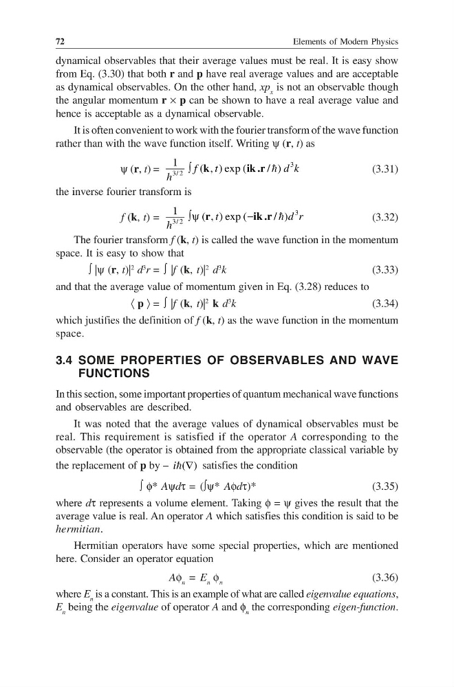
It is often convenient to work with the fourier transform of the wave function
rather than with the wave function itself. Writing ψ (r, t) as
ψ (r, t) =
3
3/ 2
1
( , ) exp (
/ )
∫
f
t
d k
h
k
i k. r
(3.31)
the inverse fourier transform is
f (k, t) =
3
3/ 2
1
( , ) exp (
/ )
∫ ψ
−
t
dr
h
r
i k. r
(3.32)
The fourier transform f (k, t) is called the wave function in the momentum
space. It is easy to show that
∫ |ψ (r, t)|
2
d
3
r = ∫ |f (k, t)|
2
d
3
k
(3.33)
and that the average value of momentum given in Eq. (3.28) reduces to
〈 p 〉 = ∫ |f (k, t)|
2
k d
3
k
(3.34)
which justifies the definition of f (k, t) as the wave function in the momentum
space.
3.4 SOME PROPERTIES OF OBSERVABLES AND WAVE
FUNCTIONS
In this section, some important properties of quantum mechanical wave functions
and observables are described.
It was noted that the average values of dynamical observables must be
real. This requirement is satisfied if the operator A corresponding to the
observable (the operator is obtained from the appropriate classical variable by
the replacement of p by – ( )
i ∇
satisfies the condition
∫ φ* Aψdτ = (∫ψ* Aφdτ)*
(3.35)
where dτ represents a volume element. Taking φ = ψ gives the result that the
average value is real. An operator A which satisfies this condition is said to be
hermitian.
Hermitian operators have some special properties, which are mentioned
here. Consider an operator equation
Aφ n = E n φ n
(3.36)
where E n is a constant. This is an example of what are called eigenvalue equations,
E n being the eigenvalue of operator A and φ n the corresponding eigen-function.
72
dynamical observables that their average values must be real. It is easy show
from Eq. (3.30) that both r and p have real average values and are acceptable
as dynamical observables. On the other hand, xp x is not an observable though
the angular momentum r × p can be shown to have a real average value and
hence is acceptable as a dynamical observable.
It is often convenient to work with the fourier transform of the wave function
rather than with the wave function itself. Writing ψ (r, t) as
ψ (r, t) =
3
3/ 2
1
( , ) exp (
/ )
∫
f
t
d k
h
k
i k. r
(3.31)
the inverse fourier transform is
f (k, t) =
3
3/ 2
1
( , ) exp (
/ )
∫ ψ
−
t
dr
h
r
i k. r
(3.32)
The fourier transform f (k, t) is called the wave function in the momentum
space. It is easy to show that
∫ |ψ (r, t)|
2
d
3
r = ∫ |f (k, t)|
2
d
3
k
(3.33)
and that the average value of momentum given in Eq. (3.28) reduces to
〈 p 〉 = ∫ |f (k, t)|
2
k d
3
k
(3.34)
which justifies the definition of f (k, t) as the wave function in the momentum
space.
3.4 SOME PROPERTIES OF OBSERVABLES AND WAVE
FUNCTIONS
In this section, some important properties of quantum mechanical wave functions
and observables are described.
It was noted that the average values of dynamical observables must be
real. This requirement is satisfied if the operator A corresponding to the
observable (the operator is obtained from the appropriate classical variable by
the replacement of p by – ( )
i ∇
satisfies the condition
∫ φ* Aψdτ = (∫ψ* Aφdτ)*
(3.35)
where dτ represents a volume element. Taking φ = ψ gives the result that the
average value is real. An operator A which satisfies this condition is said to be
hermitian.
Hermitian operators have some special properties, which are mentioned
here. Consider an operator equation
Aφ n = E n φ n
(3.36)
where E n is a constant. This is an example of what are called eigenvalue equations,
E n being the eigenvalue of operator A and φ n the corresponding eigen-function.