

Elements of Modern Physics
126
2
2
2 1/2
2
2
0
( 1) ( 1)
1
2 ( 2
/ )
2
4
r
r
n n
l l
Ze
n
m E
m
r
r
r
r
−
+
−
−
+
−
πε
= 0
(4.107)
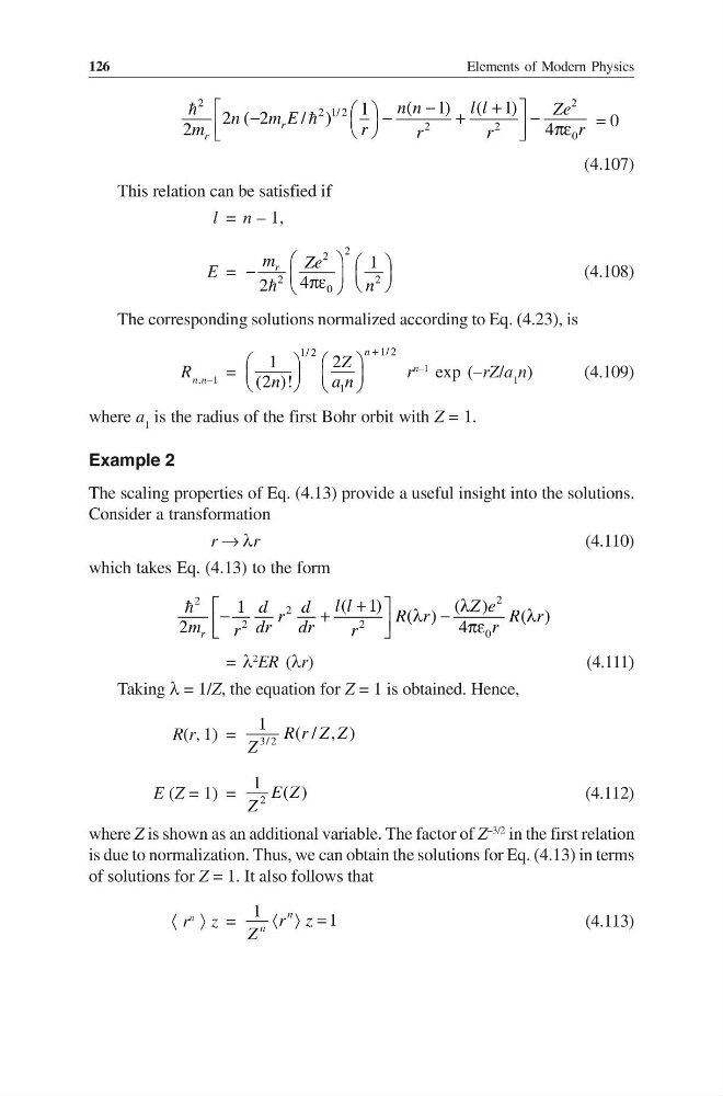
This relation can be satisfied if
l = n – 1,
E =
2
2
2
2
0
1
4
2
r
m
Ze
n
−
πε
(4.108)
The corresponding solutions normalized according to Eq. (4.23), is
R n,n–1 =
1/ 2
1/ 2
1
1
2
(2 )!
n
Z
n
an
+
r
n–1
exp (–rZ/a 1 n)
(4.109)
where a 1 is the radius of the first Bohr orbit with Z = 1.
Example 2
The scaling properties of Eq. (4.13) provide a useful insight into the solutions.
Consider a transformation
r → λr
(4.110)
which takes Eq. (4.13) to the form
2
2
2
2
2
0
( 1)
( )
1
( )
( )
2
4
r
l l
Z e
d
d
r
R r
R r
m
dr
dr
r
r
r
+
λ
−
+
λ −
λ
πε
= λ
2
ER (λr)
(4.111)
Taking λ = 1/Z, the equation for Z = 1 is obtained. Hence,
R(r, 1) = 3/ 2
1
( / , )
R r Z Z
Z
E (Z = 1) = 2
1 ( )
E Z
Z
(4.112)
where Z is shown as an additional variable. The factor of Z
–3/2
in the first relation
is due to normalization. Thus, we can obtain the solutions for Eq. (4.13) in terms
of solutions for Z = 1. It also follows that
〈 r
n
〉 z =
1
1
n
n
r z
Z
〈 〉 =
(4.113)
126
2
2
2 1/2
2
2
0
( 1) ( 1)
1
2 ( 2
/ )
2
4
r
r
n n
l l
Ze
n
m E
m
r
r
r
r
−
+
−
−
+
−
πε
= 0
(4.107)
This relation can be satisfied if
l = n – 1,
E =
2
2
2
2
0
1
4
2
r
m
Ze
n
−
πε
(4.108)
The corresponding solutions normalized according to Eq. (4.23), is
R n,n–1 =
1/ 2
1/ 2
1
1
2
(2 )!
n
Z
n
an
+
r
n–1
exp (–rZ/a 1 n)
(4.109)
where a 1 is the radius of the first Bohr orbit with Z = 1.
Example 2
The scaling properties of Eq. (4.13) provide a useful insight into the solutions.
Consider a transformation
r → λr
(4.110)
which takes Eq. (4.13) to the form
2
2
2
2
2
0
( 1)
( )
1
( )
( )
2
4
r
l l
Z e
d
d
r
R r
R r
m
dr
dr
r
r
r
+
λ
−
+
λ −
λ
πε
= λ
2
ER (λr)
(4.111)
Taking λ = 1/Z, the equation for Z = 1 is obtained. Hence,
R(r, 1) = 3/ 2
1
( / , )
R r Z Z
Z
E (Z = 1) = 2
1 ( )
E Z
Z
(4.112)
where Z is shown as an additional variable. The factor of Z
–3/2
in the first relation
is due to normalization. Thus, we can obtain the solutions for Eq. (4.13) in terms
of solutions for Z = 1. It also follows that
〈 r
n
〉 z =
1
1
n
n
r z
Z
〈 〉 =
(4.113)