

58
2 Preliminaries
0
5
10
15
20
25
0
20
40
60
80
100
x
F, g
F (x)
g(x)
x 0 = arg{g(x) = 0}
0
5
10
15
20
25
0
20
40
60
80
100
x
F, g
F (x)
g(x)
x 0 = max arg g(x) = 0}
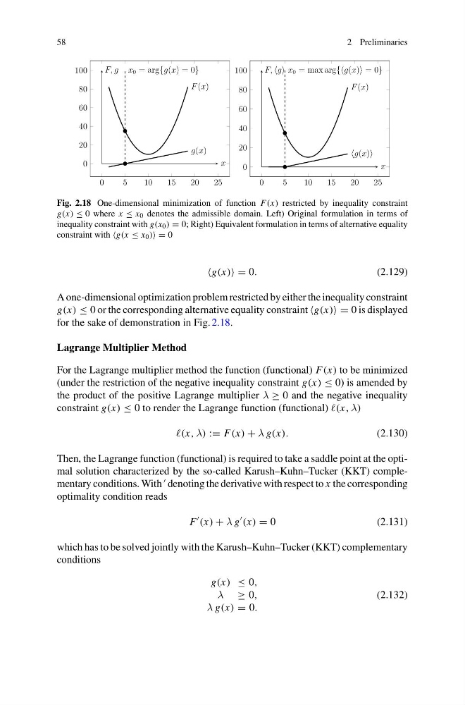
Fig. 2.18 One-dimensional minimization of function F(x) restricted by inequality constraint
g(x) ≤ 0 where x ≤ x 0 denotes the admissible domain. Left) Original formulation in terms of
inequality constraint with g(x 0 ) = 0; Right) Equivalent formulation in terms of alternative equality
constraint with ≤ x 0 ) = 0
= 0.
(2.129)
A one-dimensional optimization problem restricted by either the inequality constraint
g(x) ≤ 0 or the corresponding alternative equality constraint = 0 is displayed
for the sake of demonstration in Fig. 2.18.
Lagrange Multiplier Method
For the Lagrange multiplier method the function (functional) F(x) to be minimized
(under the restriction of the negative inequality constraint g(x) ≤ 0) is amended by
the product of the positive Lagrange multiplier λ ≥ 0 and the negative inequality
constraint g(x) ≤ 0 to render the Lagrange function (functional) λ)
λ) := F(x) + λ g(x).
(2.130)
Then, the Lagrange function (functional) is required to take a saddle point at the optimal solution characterized by the so-called Karush–Kuhn–Tucker (KKT) complementary conditions. With
denoting the derivative with respect to x the corresponding
optimality condition reads
F
(x) + λ g
(x) = 0
(2.131)
which has to be solved jointly with the Karush–Kuhn–Tucker (KKT) complementary
conditions
g(x) ≤ 0,
λ ≥ 0,
λ g(x) = 0.
(2.132)
2 Preliminaries
0
5
10
15
20
25
0
20
40
60
80
100
x
F, g
F (x)
g(x)
x 0 = arg{g(x) = 0}
0
5
10
15
20
25
0
20
40
60
80
100
x
F, g
F (x)
g(x)
x 0 = max arg g(x) = 0}
Fig. 2.18 One-dimensional minimization of function F(x) restricted by inequality constraint
g(x) ≤ 0 where x ≤ x 0 denotes the admissible domain. Left) Original formulation in terms of
inequality constraint with g(x 0 ) = 0; Right) Equivalent formulation in terms of alternative equality
constraint with ≤ x 0 ) = 0
= 0.
(2.129)
A one-dimensional optimization problem restricted by either the inequality constraint
g(x) ≤ 0 or the corresponding alternative equality constraint = 0 is displayed
for the sake of demonstration in Fig. 2.18.
Lagrange Multiplier Method
For the Lagrange multiplier method the function (functional) F(x) to be minimized
(under the restriction of the negative inequality constraint g(x) ≤ 0) is amended by
the product of the positive Lagrange multiplier λ ≥ 0 and the negative inequality
constraint g(x) ≤ 0 to render the Lagrange function (functional) λ)
λ) := F(x) + λ g(x).
(2.130)
Then, the Lagrange function (functional) is required to take a saddle point at the optimal solution characterized by the so-called Karush–Kuhn–Tucker (KKT) complementary conditions. With
denoting the derivative with respect to x the corresponding
optimality condition reads
F
(x) + λ g
(x) = 0
(2.131)
which has to be solved jointly with the Karush–Kuhn–Tucker (KKT) complementary
conditions
g(x) ≤ 0,
λ ≥ 0,
λ g(x) = 0.
(2.132)