

2.2 Computational Tools
41
material model, contribute to an archetypical structural computation. Obviously, the
one-dimensional, geometrically linear setting is normally not sufficient for real world
analyses without extension to multiple dimensions; however, it already contains all
the main ingredients characterizing structural analyses without requiring mastering
the algebraically challenging multi-dimensional setting.
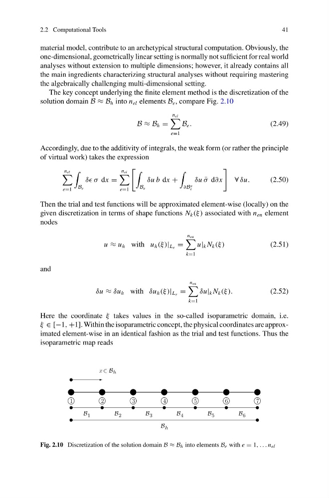
The key concept underlying the finite element method is the discretization of the
solution domain B ≈ B h into n el elements B e , compare Fig. 2.10
B ≈ B h =
n el
e=1
B e .
(2.49)
Accordingly, due to the additivity of integrals, the weak form (or rather the principle
of virtual work) takes the expression
n el
e=1
B e
δδ σ dx =
n el
e=1
B e
δu b dx +
∂B σ
e
δu ¯
σ d∂ x
∀ δu.
(2.50)
Then the trial and test functions will be approximated element-wise (locally) on the
given discretization in terms of shape functions N k (ξ ) associated with n en element
nodes
u ≈ u h with u h (ξ )| L e =
n en
k=1
u| k N k (ξ )
(2.51)
and
δu ≈ δu h with δu h (ξ )| L e =
n en
k=1
δu| k N k (ξ ).
(2.52)
Here the coordinate ξ takes values in the so-called isoparametric domain, i.e.
ξ ∈ [−1, +1]. Within the isoparametric concept, the physical coordinates are approximated element-wise in an identical fashion as the trial and test functions. Thus the
isoparametric map reads
B h
1
2
3
4
5
6
7
B 1
B 2
B 3
B 4
B 5
B 6
x ∈ B h
Fig. 2.10 Discretization of the solution domain B ≈ B h into elements B e with e = 1, . . . n el
41
material model, contribute to an archetypical structural computation. Obviously, the
one-dimensional, geometrically linear setting is normally not sufficient for real world
analyses without extension to multiple dimensions; however, it already contains all
the main ingredients characterizing structural analyses without requiring mastering
the algebraically challenging multi-dimensional setting.
The key concept underlying the finite element method is the discretization of the
solution domain B ≈ B h into n el elements B e , compare Fig. 2.10
B ≈ B h =
n el
e=1
B e .
(2.49)
Accordingly, due to the additivity of integrals, the weak form (or rather the principle
of virtual work) takes the expression
n el
e=1
B e
δδ σ dx =
n el
e=1
B e
δu b dx +
∂B σ
e
δu ¯
σ d∂ x
∀ δu.
(2.50)
Then the trial and test functions will be approximated element-wise (locally) on the
given discretization in terms of shape functions N k (ξ ) associated with n en element
nodes
u ≈ u h with u h (ξ )| L e =
n en
k=1
u| k N k (ξ )
(2.51)
and
δu ≈ δu h with δu h (ξ )| L e =
n en
k=1
δu| k N k (ξ ).
(2.52)
Here the coordinate ξ takes values in the so-called isoparametric domain, i.e.
ξ ∈ [−1, +1]. Within the isoparametric concept, the physical coordinates are approximated element-wise in an identical fashion as the trial and test functions. Thus the
isoparametric map reads
B h
1
2
3
4
5
6
7
B 1
B 2
B 3
B 4
B 5
B 6
x ∈ B h
Fig. 2.10 Discretization of the solution domain B ≈ B h into elements B e with e = 1, . . . n el