

340
6 Visco-Plasticity
π
∗
(σ vp , σ hi ) =
⎧
⎪ ⎪ ⎨
⎪ ⎪ ⎩
0
|σ vp | < σ y − σ hi
for
1
2
|σ vp | − [σ y − σ hi ]
2
η
|σ vp | ≥ σ y − σ hi
⎫
⎪ ⎪ ⎬
⎪ ⎪ ⎭
.
(6.141)
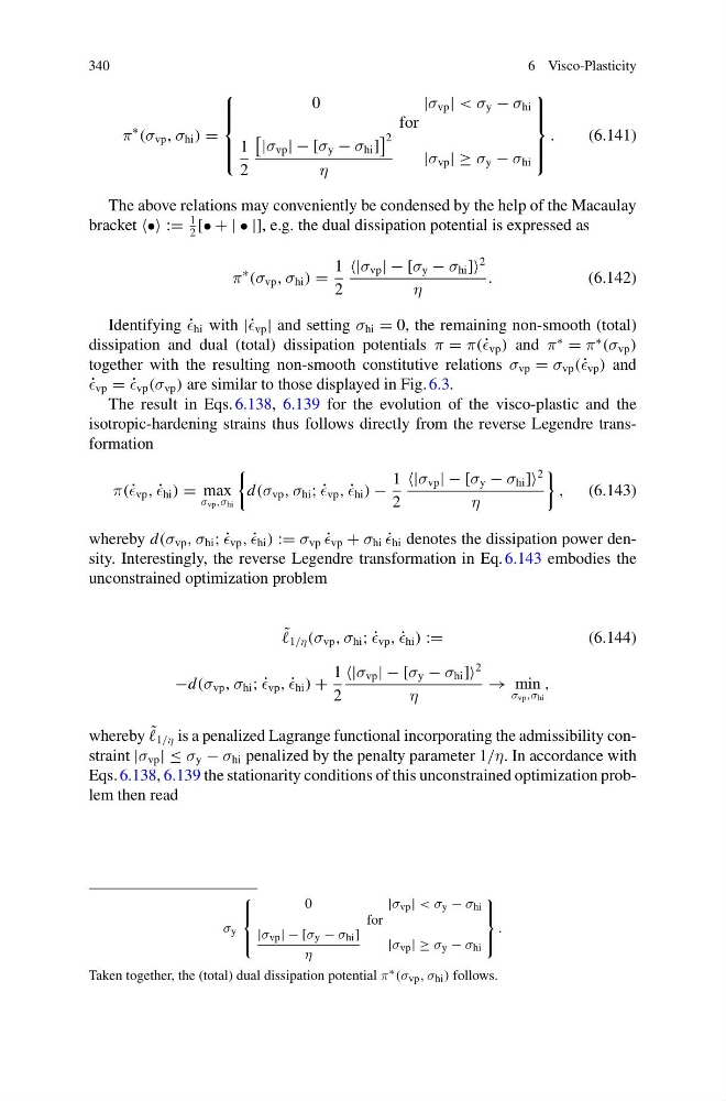
The above relations may conveniently be condensed by the help of the Macaulay
bracket :=
1
2
[• + | • |], e.g. the dual dissipation potential is expressed as
π
∗
(σ vp , σ hi ) =
1
2
|σ vp | − [σ y − σ hi ]]
2
η
.
(6.142)
Identifying ˙
hi with |˙ vp | and setting σ hi = 0, the remaining non-smooth (total)
dissipation and dual (total) dissipation potentials π = π(˙ vp ) and π
∗
= π
∗
(σ vp )
together with the resulting non-smooth constitutive relations σ vp = σ vp (˙ vp ) and
˙
vp = ˙
vp (σ vp ) are similar to those displayed in Fig. 6.3.
The result in Eqs. 6.138, 6.139 for the evolution of the visco-plastic and the
isotropic-hardening strains thus follows directly from the reverse Legendre transformation
π(˙ vp , ˙
hi ) = max
σ vp ,σ hi
d(σ vp , σ hi ; ˙
vp , ˙
hi ) −
1
2
|σ vp | − [σ y − σ hi ]]
2
η
, (6.143)
whereby d(σ vp , σ hi ; ˙
vp , ˙
hi ) := σ vp ˙
vp + σ hi ˙
hi denotes the dissipation power density. Interestingly, the reverse Legendre transformation in Eq. 6.143 embodies the
unconstrained optimization problem
˜
1/η (σ vp , σ hi ; ˙
vp , ˙
hi ) :=
(6.144)
−d(σ vp , σ hi ; ˙
vp , ˙
hi ) +
1
2
|σ vp | − [σ y − σ hi ]]
2
η
→ min
σ vp ,σ hi
,
whereby ˜
1/η is a penalized Lagrange functional incorporating the admissibility constraint |σ vp | ≤ σ y − σ hi penalized by the penalty parameter 1/η. In accordance with
Eqs. 6.138, 6.139 the stationarity conditions of this unconstrained optimization problem then read
σ y
⎧
⎪ ⎨
⎪ ⎩
0
|σ vp | < σ y − σ hi
for
|σ vp | − [σ y − σ hi ]
η
|σ vp | ≥ σ y − σ hi
⎫
⎪ ⎬
⎪ ⎭
.
Taken together, the (total) dual dissipation potential π ∗ (σ vp , σ hi ) follows.
6 Visco-Plasticity
π
∗
(σ vp , σ hi ) =
⎧
⎪ ⎪ ⎨
⎪ ⎪ ⎩
0
|σ vp | < σ y − σ hi
for
1
2
|σ vp | − [σ y − σ hi ]
2
η
|σ vp | ≥ σ y − σ hi
⎫
⎪ ⎪ ⎬
⎪ ⎪ ⎭
.
(6.141)
The above relations may conveniently be condensed by the help of the Macaulay
bracket :=
1
2
[• + | • |], e.g. the dual dissipation potential is expressed as
π
∗
(σ vp , σ hi ) =
1
2
|σ vp | − [σ y − σ hi ]]
2
η
.
(6.142)
Identifying ˙
hi with |˙ vp | and setting σ hi = 0, the remaining non-smooth (total)
dissipation and dual (total) dissipation potentials π = π(˙ vp ) and π
∗
= π
∗
(σ vp )
together with the resulting non-smooth constitutive relations σ vp = σ vp (˙ vp ) and
˙
vp = ˙
vp (σ vp ) are similar to those displayed in Fig. 6.3.
The result in Eqs. 6.138, 6.139 for the evolution of the visco-plastic and the
isotropic-hardening strains thus follows directly from the reverse Legendre transformation
π(˙ vp , ˙
hi ) = max
σ vp ,σ hi
d(σ vp , σ hi ; ˙
vp , ˙
hi ) −
1
2
|σ vp | − [σ y − σ hi ]]
2
η
, (6.143)
whereby d(σ vp , σ hi ; ˙
vp , ˙
hi ) := σ vp ˙
vp + σ hi ˙
hi denotes the dissipation power density. Interestingly, the reverse Legendre transformation in Eq. 6.143 embodies the
unconstrained optimization problem
˜
1/η (σ vp , σ hi ; ˙
vp , ˙
hi ) :=
(6.144)
−d(σ vp , σ hi ; ˙
vp , ˙
hi ) +
1
2
|σ vp | − [σ y − σ hi ]]
2
η
→ min
σ vp ,σ hi
,
whereby ˜
1/η is a penalized Lagrange functional incorporating the admissibility constraint |σ vp | ≤ σ y − σ hi penalized by the penalty parameter 1/η. In accordance with
Eqs. 6.138, 6.139 the stationarity conditions of this unconstrained optimization problem then read
σ y
⎧
⎪ ⎨
⎪ ⎩
0
|σ vp | < σ y − σ hi
for
|σ vp | − [σ y − σ hi ]
η
|σ vp | ≥ σ y − σ hi
⎫
⎪ ⎬
⎪ ⎭
.
Taken together, the (total) dual dissipation potential π ∗ (σ vp , σ hi ) follows.