

320
6 Visco-Plasticity
As a conclusion the algorithmic tangent E a is thus finally expressed as
E
n
a = E − H 0 ((λ)
E
2
E + η//t n .
(6.107)
Note that, consequently, the algorithmic tangent degenerates to E a = 0 for η → 0
and λ > 0, likewise it degenerates to E a = E for t
n
→ 0. In one dimension the
algorithmic tangent trivially coincides with its continuous counterpart. It shall be
noted, however, that this is at variance with the corresponding result in two and three
dimensions.
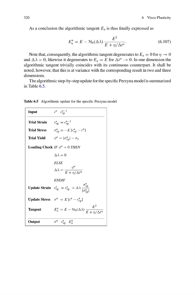
The algorithmic step-by-step update for the specific Perzyna model is summarized
in Table 6.5.
Table 6.5 Algorithmic update for the specific Perzyna model
Input
n n−1
vp
Trial Strain
vp = n−1
vp
Trial Stress
σ
vp = −E [
vp − n ]
Trial Yield
φ = |σ
vp | − σ y
Loading Check IF φ < 0 THEN
λ = 0
ELSE
λ =
φ
E + η//t n
ENDIF
Update Strain n
vp =
vp + λ
σ
vp
|σ
vp |
Update Stress σ n = E [ n − n
vp ]
Tangent
E n
a = E − H 0 ((λ)
E 2
E + η//t n
Output
σ n n
vp E n
a
6 Visco-Plasticity
As a conclusion the algorithmic tangent E a is thus finally expressed as
E
n
a = E − H 0 ((λ)
E
2
E + η//t n .
(6.107)
Note that, consequently, the algorithmic tangent degenerates to E a = 0 for η → 0
and λ > 0, likewise it degenerates to E a = E for t
n
→ 0. In one dimension the
algorithmic tangent trivially coincides with its continuous counterpart. It shall be
noted, however, that this is at variance with the corresponding result in two and three
dimensions.
The algorithmic step-by-step update for the specific Perzyna model is summarized
in Table 6.5.
Table 6.5 Algorithmic update for the specific Perzyna model
Input
n n−1
vp
Trial Strain
vp = n−1
vp
Trial Stress
σ
vp = −E [
vp − n ]
Trial Yield
φ = |σ
vp | − σ y
Loading Check IF φ < 0 THEN
λ = 0
ELSE
λ =
φ
E + η//t n
ENDIF
Update Strain n
vp =
vp + λ
σ
vp
|σ
vp |
Update Stress σ n = E [ n − n
vp ]
Tangent
E n
a = E − H 0 ((λ)
E 2
E + η//t n
Output
σ n n
vp E n
a