

282
5 Plasticity
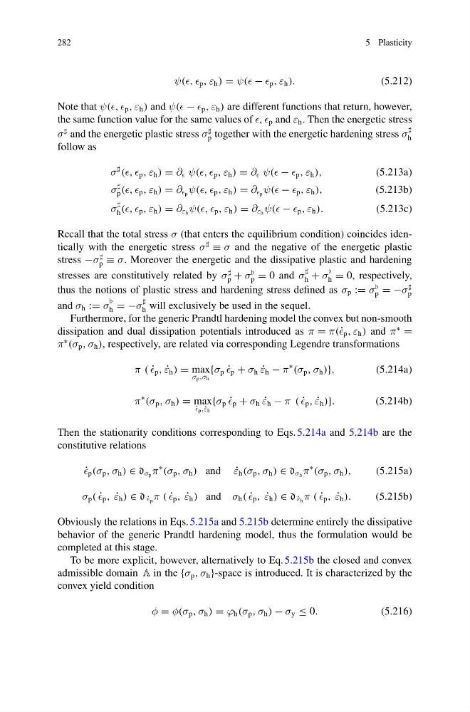
ψ(, p , ε h ) = ψ( − p , ε h ).
(5.212)
Note that ψ(, p , ε h ) and ψ( − p , ε h ) are different functions that return, however,
the same function value for the same values of , p and ε h . Then the energetic stress
σ
and the energetic plastic stress σ
p together with the energetic hardening stress σ
h
follow as
σ
(, p , ε h ) = ∂ ψ(, p , ε h ) = ∂ ψ( − p , ε h ),
(5.213a)
σ
p (, p , ε h ) = ∂ p ψ(, p , ε h ) = ∂ p ψ( − p , ε h ),
(5.213b)
σ
h (, p , ε h ) = ∂ ε h ψ(, p , ε h ) = ∂ ε h ψ( − p , ε h ).
(5.213c)
Recall that the total stress σ (that enters the equilibrium condition) coincides identically with the energetic stress σ
≡ σ and the negative of the energetic plastic
stress −σ
p ≡ σ. Moreover the energetic and the dissipative plastic and hardening
stresses are constitutively related by σ
p + σ
p = 0 and σ
h + σ
h = 0, respectively,
thus the notions of plastic stress and hardening stress defined as σ p := σ
p = −σ
p
and σ h := σ
h = −σ
h will exclusively be used in the sequel.
Furthermore, for the generic Prandtl hardening model the convex but non-smooth
dissipation and dual dissipation potentials introduced as π = π(˙ p , ε h ) and π
∗
=
π
∗
(σ p , σ h ), respectively, are related via corresponding Legendre transformations
π ( ˙
p , ˙
ε h ) = max
σ p ,σ h
{σ p ˙
p + σ h ˙
ε h − π
∗
(σ p , σ h )},
(5.214a)
π
∗
(σ p , σ h ) = max
˙
p ,˙ ε h
{σ p ˙
p + σ h ˙
ε h − π ( ˙
p , ˙
ε h )}.
(5.214b)
Then the stationarity conditions corresponding to Eqs. 5.214a and 5.214b are the
constitutive relations
˙
p (σ p , σ h ) ∈ d σ p π
∗
(σ p , σ h ) and ˙
ε h (σ p , σ h ) ∈ d σ h π
∗
(σ p , σ h ),
(5.215a)
σ p ( ˙
p , ˙
ε h ) ∈ d ˙
p π ( ˙
p , ˙
ε h ) and σ h ( ˙
p , ˙
ε h ) ∈ d ˙
ε h π ( ˙
p , ˙
ε h ).
(5.215b)
Obviously the relations in Eqs. 5.215a and 5.215b determine entirely the dissipative
behavior of the generic Prandtl hardening model, thus the formulation would be
completed at this stage.
To be more explicit, however, alternatively to Eq. 5.215b the closed and convex
admissible domain A in the {σ p , σ h }-space is introduced. It is characterized by the
convex yield condition
φ = φ(σ p , σ h ) = ϕ h (σ p , σ h ) − σ y ≤ 0.
(5.216)
5 Plasticity
ψ(, p , ε h ) = ψ( − p , ε h ).
(5.212)
Note that ψ(, p , ε h ) and ψ( − p , ε h ) are different functions that return, however,
the same function value for the same values of , p and ε h . Then the energetic stress
σ
and the energetic plastic stress σ
p together with the energetic hardening stress σ
h
follow as
σ
(, p , ε h ) = ∂ ψ(, p , ε h ) = ∂ ψ( − p , ε h ),
(5.213a)
σ
p (, p , ε h ) = ∂ p ψ(, p , ε h ) = ∂ p ψ( − p , ε h ),
(5.213b)
σ
h (, p , ε h ) = ∂ ε h ψ(, p , ε h ) = ∂ ε h ψ( − p , ε h ).
(5.213c)
Recall that the total stress σ (that enters the equilibrium condition) coincides identically with the energetic stress σ
≡ σ and the negative of the energetic plastic
stress −σ
p ≡ σ. Moreover the energetic and the dissipative plastic and hardening
stresses are constitutively related by σ
p + σ
p = 0 and σ
h + σ
h = 0, respectively,
thus the notions of plastic stress and hardening stress defined as σ p := σ
p = −σ
p
and σ h := σ
h = −σ
h will exclusively be used in the sequel.
Furthermore, for the generic Prandtl hardening model the convex but non-smooth
dissipation and dual dissipation potentials introduced as π = π(˙ p , ε h ) and π
∗
=
π
∗
(σ p , σ h ), respectively, are related via corresponding Legendre transformations
π ( ˙
p , ˙
ε h ) = max
σ p ,σ h
{σ p ˙
p + σ h ˙
ε h − π
∗
(σ p , σ h )},
(5.214a)
π
∗
(σ p , σ h ) = max
˙
p ,˙ ε h
{σ p ˙
p + σ h ˙
ε h − π ( ˙
p , ˙
ε h )}.
(5.214b)
Then the stationarity conditions corresponding to Eqs. 5.214a and 5.214b are the
constitutive relations
˙
p (σ p , σ h ) ∈ d σ p π
∗
(σ p , σ h ) and ˙
ε h (σ p , σ h ) ∈ d σ h π
∗
(σ p , σ h ),
(5.215a)
σ p ( ˙
p , ˙
ε h ) ∈ d ˙
p π ( ˙
p , ˙
ε h ) and σ h ( ˙
p , ˙
ε h ) ∈ d ˙
ε h π ( ˙
p , ˙
ε h ).
(5.215b)
Obviously the relations in Eqs. 5.215a and 5.215b determine entirely the dissipative
behavior of the generic Prandtl hardening model, thus the formulation would be
completed at this stage.
To be more explicit, however, alternatively to Eq. 5.215b the closed and convex
admissible domain A in the {σ p , σ h }-space is introduced. It is characterized by the
convex yield condition
φ = φ(σ p , σ h ) = ϕ h (σ p , σ h ) − σ y ≤ 0.
(5.216)