

5.3 Prandtl Hardening Model
271
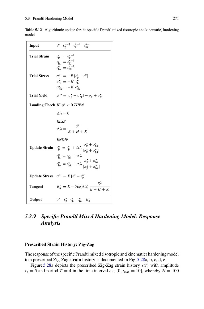
Table 5.12 Algorithmic update for the specific Prandtl mixed (isotropic and kinematic) hardening
model
Input
n n−1
p
n−1
hi
n−1
hk
Trial Strain
p = n−1
p
hi =
n−1
hi
hk =
n−1
hk
Trial Stress
σ
p = −E [
p − n ]
σ
hi = −H
hi
σ
hk = −K
hk
Trial Yield
φ = |σ
p + σ
hk | − σ y + σ
hi
Loading Check IF φ < 0 THEN
λ = 0
ELSE
λ =
φ
E + H + K
ENDIF
Update Strain n
p =
p + λ
σ
p + σ
hk
|σ
p + σ
hk |
n
hi =
hi + λ
n
hk =
hk + λ
σ
p + σ
hk
|σ
p + σ
hk |
Update Stress σ n = E [ n − n
p ]
Tangent
E n
a = E − H 0 ((λ)
E 2
E + H + K
Output
σ n n
p
n
hi
n
hk E n
a
5.3.9 Specific Prandtl Mixed Hardening Model: Response
Analysis
Prescribed Strain History: Zig-Zag
The response of the specific Prandtl mixed (isotropic and kinematic) hardening model
to a prescribed Zig-Zag strain history is documented in Fig. 5.28a, b, c, d, e.
Figure 5.28a depicts the prescribed Zig-Zag strain history (t) with amplitude
a = 5 and period T = 4 in the time interval t ∈ [0, t max = 10], whereby N = 100
271
Table 5.12 Algorithmic update for the specific Prandtl mixed (isotropic and kinematic) hardening
model
Input
n n−1
p
n−1
hi
n−1
hk
Trial Strain
p = n−1
p
hi =
n−1
hi
hk =
n−1
hk
Trial Stress
σ
p = −E [
p − n ]
σ
hi = −H
hi
σ
hk = −K
hk
Trial Yield
φ = |σ
p + σ
hk | − σ y + σ
hi
Loading Check IF φ < 0 THEN
λ = 0
ELSE
λ =
φ
E + H + K
ENDIF
Update Strain n
p =
p + λ
σ
p + σ
hk
|σ
p + σ
hk |
n
hi =
hi + λ
n
hk =
hk + λ
σ
p + σ
hk
|σ
p + σ
hk |
Update Stress σ n = E [ n − n
p ]
Tangent
E n
a = E − H 0 ((λ)
E 2
E + H + K
Output
σ n n
p
n
hi
n
hk E n
a
5.3.9 Specific Prandtl Mixed Hardening Model: Response
Analysis
Prescribed Strain History: Zig-Zag
The response of the specific Prandtl mixed (isotropic and kinematic) hardening model
to a prescribed Zig-Zag strain history is documented in Fig. 5.28a, b, c, d, e.
Figure 5.28a depicts the prescribed Zig-Zag strain history (t) with amplitude
a = 5 and period T = 4 in the time interval t ∈ [0, t max = 10], whereby N = 100