

5.3 Prandtl Hardening Model
269
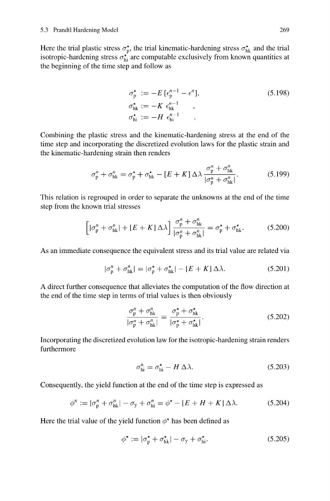
Here the trial plastic stress σ
p , the trial kinematic-hardening stress σ
hk and the trial
isotropic-hardening stress σ
hi are computable exclusively from known quantities at
the beginning of the time step and follow as
σ
p := −E [
n−1
p
−
n
],
(5.198)
σ
hk := −K
n−1
hk
,
σ
hi := −H
n−1
hi
.
Combining the plastic stress and the kinematic-hardening stress at the end of the
time step and incorporating the discretized evolution laws for the plastic strain and
the kinematic-hardening strain then renders
σ
n
p + σ
n
hk = σ
p + σ
hk − [E + K ] λ
σ
n
p + σ
n
hk
|σ n
p + σ
n
hk |
.
(5.199)
This relation is regrouped in order to separate the unknowns at the end of the time
step from the known trial stresses
|σ
n
p + σ
n
hk | + [E + K ] λ
σ
n
p + σ
n
hk
|σ n
p + σ
n
hk |
= σ
p + σ
hk .
(5.200)
As an immediate consequence the equivalent stress and its trial value are related via
|σ
n
p + σ
n
hk | = |σ
p + σ
hk | − [E + K ] λ.
(5.201)
A direct further consequence that alleviates the computation of the flow direction at
the end of the time step in terms of trial values is then obviously
σ
n
p + σ
n
hk
|σ n
p + σ
n
hk |
≡
σ
p + σ
hk
|σ
p + σ
hk |
.
(5.202)
Incorporating the discretized evolution law for the isotropic-hardening strain renders
furthermore
σ
n
hi = σ
hi − H λ.
(5.203)
Consequently, the yield function at the end of the time step is expressed as
φ
n
:= |σ
n
p + σ
n
hk | − σ y + σ
n
hi = φ
− [E + H + K ] λ.
(5.204)
Here the trial value of the yield function φ
has been defined as
φ
:= |σ
p + σ
hk | − σ y + σ
hi .
(5.205)
269
Here the trial plastic stress σ
p , the trial kinematic-hardening stress σ
hk and the trial
isotropic-hardening stress σ
hi are computable exclusively from known quantities at
the beginning of the time step and follow as
σ
p := −E [
n−1
p
−
n
],
(5.198)
σ
hk := −K
n−1
hk
,
σ
hi := −H
n−1
hi
.
Combining the plastic stress and the kinematic-hardening stress at the end of the
time step and incorporating the discretized evolution laws for the plastic strain and
the kinematic-hardening strain then renders
σ
n
p + σ
n
hk = σ
p + σ
hk − [E + K ] λ
σ
n
p + σ
n
hk
|σ n
p + σ
n
hk |
.
(5.199)
This relation is regrouped in order to separate the unknowns at the end of the time
step from the known trial stresses
|σ
n
p + σ
n
hk | + [E + K ] λ
σ
n
p + σ
n
hk
|σ n
p + σ
n
hk |
= σ
p + σ
hk .
(5.200)
As an immediate consequence the equivalent stress and its trial value are related via
|σ
n
p + σ
n
hk | = |σ
p + σ
hk | − [E + K ] λ.
(5.201)
A direct further consequence that alleviates the computation of the flow direction at
the end of the time step in terms of trial values is then obviously
σ
n
p + σ
n
hk
|σ n
p + σ
n
hk |
≡
σ
p + σ
hk
|σ
p + σ
hk |
.
(5.202)
Incorporating the discretized evolution law for the isotropic-hardening strain renders
furthermore
σ
n
hi = σ
hi − H λ.
(5.203)
Consequently, the yield function at the end of the time step is expressed as
φ
n
:= |σ
n
p + σ
n
hk | − σ y + σ
n
hi = φ
− [E + H + K ] λ.
(5.204)
Here the trial value of the yield function φ
has been defined as
φ
:= |σ
p + σ
hk | − σ y + σ
hi .
(5.205)