

5.3 Prandtl Hardening Model
249
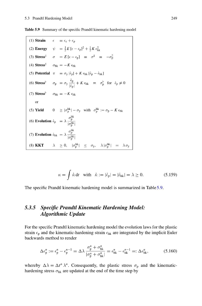
Table 5.9 Summary of the specific Prandtl kinematic hardening model
(1) Strain
= e + p
(2) Energy ψ =
1
2 E [ − p ] 2 +
1
2 K 2
hk
(3) Stress
σ = E [ − p ] ≡ σ ≡ −σ
p
(4) Stress
σ hk = −K hk
(5) Potential π = σ y |˙ p | + K hk [˙ p − ˙
hk ]
(6) Stress
σ p = σ y
˙
p
|˙ p |
+ K hk ≡ σ
p for ˙
p = 0
(7) Stress
σ hk = −K hk
or
(5) Yield
0 ≥ |σ hk
p | − σ y with σ hk
p := σ p − K hk
(6) Evolution ˙
p = λ
σ hk
p
|σ hk
p |
(7) Evolution ˙
hk = λ
σ hk
p
|σ hk
p |
(8) KKT
λ ≥ 0, |σ hk
p | ≤ σ y , λ |σ hk
p | = λ σ y
κ =
˙
κ dt with ˙
κ := |˙ p | = |˙ hk | = λ ≥ 0.
(5.159)
The specific Prandtl kinematic hardening model is summarized in Table 5.9.
5.3.5 Specific Prandtl Kinematic Hardening Model:
Algorithmic Update
For the specific Prandtl kinematic hardening model the evolution laws for the plastic
strain p and the kinematic-hardening strain hk are integrated by the implicit Euler
backwards method to render
n
p :=
n
p −
n−1
p
= λ
σ
n
p + σ
n
hk
|σ n
p + σ
n
hk |
=
n
hk −
n−1
hk =:
n
hk ,
(5.160)
whereby λ = t
n
λ
n . Consequently, the plastic stress σ p and the kinematichardening stress σ hk are updated at the end of the time step by
249
Table 5.9 Summary of the specific Prandtl kinematic hardening model
(1) Strain
= e + p
(2) Energy ψ =
1
2 E [ − p ] 2 +
1
2 K 2
hk
(3) Stress
σ = E [ − p ] ≡ σ ≡ −σ
p
(4) Stress
σ hk = −K hk
(5) Potential π = σ y |˙ p | + K hk [˙ p − ˙
hk ]
(6) Stress
σ p = σ y
˙
p
|˙ p |
+ K hk ≡ σ
p for ˙
p = 0
(7) Stress
σ hk = −K hk
or
(5) Yield
0 ≥ |σ hk
p | − σ y with σ hk
p := σ p − K hk
(6) Evolution ˙
p = λ
σ hk
p
|σ hk
p |
(7) Evolution ˙
hk = λ
σ hk
p
|σ hk
p |
(8) KKT
λ ≥ 0, |σ hk
p | ≤ σ y , λ |σ hk
p | = λ σ y
κ =
˙
κ dt with ˙
κ := |˙ p | = |˙ hk | = λ ≥ 0.
(5.159)
The specific Prandtl kinematic hardening model is summarized in Table 5.9.
5.3.5 Specific Prandtl Kinematic Hardening Model:
Algorithmic Update
For the specific Prandtl kinematic hardening model the evolution laws for the plastic
strain p and the kinematic-hardening strain hk are integrated by the implicit Euler
backwards method to render
n
p :=
n
p −
n−1
p
= λ
σ
n
p + σ
n
hk
|σ n
p + σ
n
hk |
=
n
hk −
n−1
hk =:
n
hk ,
(5.160)
whereby λ = t
n
λ
n . Consequently, the plastic stress σ p and the kinematichardening stress σ hk are updated at the end of the time step by