

228
5 Plasticity
H
H
hi
σ p
0
+σ y
σ p = +σ y +
hi
−σ y
σ p = −σ y −
hi
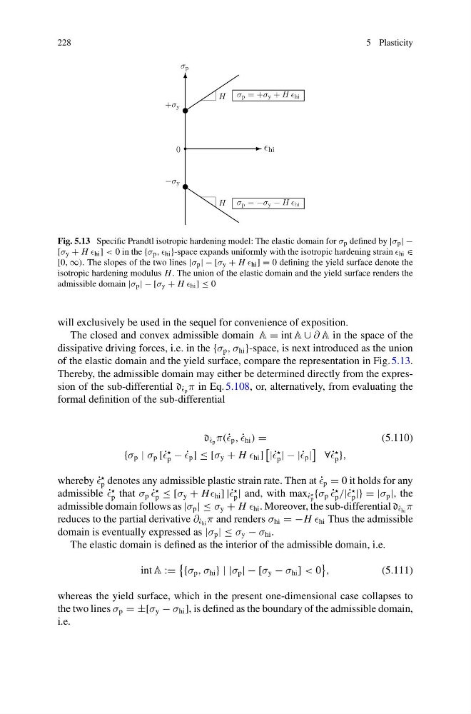
Fig. 5.13 Specific Prandtl isotropic hardening model: The elastic domain for σ p defined by |σ p | −
[σ y + H hi ] < 0 in the {σ p , hi }-space expands uniformly with the isotropic hardening strain hi ∈
[0, ∞). The slopes of the two lines |σ p | − [σ y + H hi ] = 0 defining the yield surface denote the
isotropic hardening modulus H . The union of the elastic domain and the yield surface renders the
admissible domain |σ p | − [σ y + H hi ] ≤ 0
will exclusively be used in the sequel for convenience of exposition.
The closed and convex admissible domain A = int A ∪ ∂ A in the space of the
dissipative driving forces, i.e. in the {σ p , σ hi }-space, is next introduced as the union
of the elastic domain and the yield surface, compare the representation in Fig. 5.13.
Thereby, the admissible domain may either be determined directly from the expression of the sub-differential d ˙
p π in Eq. 5.108, or, alternatively, from evaluating the
formal definition of the sub-differential
d ˙
p π(˙ p , ˙
hi ) =
(5.110)
{σ p | σ p [˙
p − ˙
p ] ≤ [σ y + H hi ]
|˙
p | − |˙ p |
∀˙
p },
whereby ˙
p denotes any admissible plastic strain rate. Then at ˙
p = 0 it holds for any
admissible ˙
p that σ p ˙
p ≤ [σ y + H hi ] |˙
p | and, with max ˙
p
{σ p ˙
p /|˙
p |} = |σ p |, the
admissible domain follows as |σ p | ≤ σ y + H hi . Moreover, the sub-differential d ˙
hi π
reduces to the partial derivative ∂ ˙
hi π and renders σ hi = −H hi Thus the admissible
domain is eventually expressed as |σ p | ≤ σ y − σ hi .
The elastic domain is defined as the interior of the admissible domain, i.e.
int A :=
{σ p , σ hi } | |σ p | − [σ y − σ hi ] < 0
,
(5.111)
whereas the yield surface, which in the present one-dimensional case collapses to
the two lines σ p = ±[σ y − σ hi ], is defined as the boundary of the admissible domain,
i.e.
5 Plasticity
H
H
hi
σ p
0
+σ y
σ p = +σ y +
hi
−σ y
σ p = −σ y −
hi
Fig. 5.13 Specific Prandtl isotropic hardening model: The elastic domain for σ p defined by |σ p | −
[σ y + H hi ] < 0 in the {σ p , hi }-space expands uniformly with the isotropic hardening strain hi ∈
[0, ∞). The slopes of the two lines |σ p | − [σ y + H hi ] = 0 defining the yield surface denote the
isotropic hardening modulus H . The union of the elastic domain and the yield surface renders the
admissible domain |σ p | − [σ y + H hi ] ≤ 0
will exclusively be used in the sequel for convenience of exposition.
The closed and convex admissible domain A = int A ∪ ∂ A in the space of the
dissipative driving forces, i.e. in the {σ p , σ hi }-space, is next introduced as the union
of the elastic domain and the yield surface, compare the representation in Fig. 5.13.
Thereby, the admissible domain may either be determined directly from the expression of the sub-differential d ˙
p π in Eq. 5.108, or, alternatively, from evaluating the
formal definition of the sub-differential
d ˙
p π(˙ p , ˙
hi ) =
(5.110)
{σ p | σ p [˙
p − ˙
p ] ≤ [σ y + H hi ]
|˙
p | − |˙ p |
∀˙
p },
whereby ˙
p denotes any admissible plastic strain rate. Then at ˙
p = 0 it holds for any
admissible ˙
p that σ p ˙
p ≤ [σ y + H hi ] |˙
p | and, with max ˙
p
{σ p ˙
p /|˙
p |} = |σ p |, the
admissible domain follows as |σ p | ≤ σ y + H hi . Moreover, the sub-differential d ˙
hi π
reduces to the partial derivative ∂ ˙
hi π and renders σ hi = −H hi Thus the admissible
domain is eventually expressed as |σ p | ≤ σ y − σ hi .
The elastic domain is defined as the interior of the admissible domain, i.e.
int A :=
{σ p , σ hi } | |σ p | − [σ y − σ hi ] < 0
,
(5.111)
whereas the yield surface, which in the present one-dimensional case collapses to
the two lines σ p = ±[σ y − σ hi ], is defined as the boundary of the admissible domain,
i.e.