

4.5 Generalized-Maxwell Model
167
σ
σ
e
v
E ∞
E m
η m
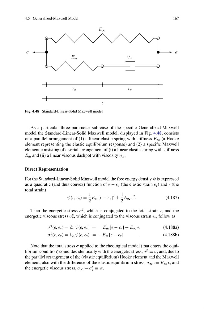
Fig. 4.48 Standard-Linear-Solid Maxwell model
As a particular three parameter sub-case of the specific Generalized-Maxwell
model the Standard-Linear-Solid Maxwell model, displayed in Fig. 4.48, consists
of a parallel arrangement of (1) a linear elastic spring with stiffness E ∞ (a Hooke
element representing the elastic equilibrium response) and (2) a specific Maxwell
element consisting of a serial arrangement of (i) a linear elastic spring with stiffness
E m and (ii) a linear viscous dashpot with viscosity η m .
Direct Representation
For the Standard-Linear-Solid Maxwell model the free energy density ψ is expressed
as a quadratic (and thus convex) function of − v (the elastic strain e ) and (the
total strain)
ψ( v ) =
1
2
E m [ − v ]
2
+
1
2
E ∞
2
.
(4.187)
Then the energetic stress σ
, which is conjugated to the total strain , and the
energetic viscous stress σ
v , which is conjugated to the viscous strain v , follow as
σ
( v ) = ∂ ψ( v ) =
E m [ − v ] + E ∞
(4.188a)
σ
v ( v ) = ∂ v ψ( v ) = −E m [ − v ]
.
(4.188b)
Note that the total stress σ applied to the rheological model (that enters the equilibrium condition) coincides identically with the energetic stress, σ
≡ σ, and, due to
the parallel arrangement of the (elastic equilibrium) Hooke element and the Maxwell
element, also with the difference of the elastic equilibrium stress, σ ∞ := E ∞ , and
the energetic viscous stress, σ ∞ − σ
v ≡ σ.
167
σ
σ
e
v
E ∞
E m
η m
Fig. 4.48 Standard-Linear-Solid Maxwell model
As a particular three parameter sub-case of the specific Generalized-Maxwell
model the Standard-Linear-Solid Maxwell model, displayed in Fig. 4.48, consists
of a parallel arrangement of (1) a linear elastic spring with stiffness E ∞ (a Hooke
element representing the elastic equilibrium response) and (2) a specific Maxwell
element consisting of a serial arrangement of (i) a linear elastic spring with stiffness
E m and (ii) a linear viscous dashpot with viscosity η m .
Direct Representation
For the Standard-Linear-Solid Maxwell model the free energy density ψ is expressed
as a quadratic (and thus convex) function of − v (the elastic strain e ) and (the
total strain)
ψ( v ) =
1
2
E m [ − v ]
2
+
1
2
E ∞
2
.
(4.187)
Then the energetic stress σ
, which is conjugated to the total strain , and the
energetic viscous stress σ
v , which is conjugated to the viscous strain v , follow as
σ
( v ) = ∂ ψ( v ) =
E m [ − v ] + E ∞
(4.188a)
σ
v ( v ) = ∂ v ψ( v ) = −E m [ − v ]
.
(4.188b)
Note that the total stress σ applied to the rheological model (that enters the equilibrium condition) coincides identically with the energetic stress, σ
≡ σ, and, due to
the parallel arrangement of the (elastic equilibrium) Hooke element and the Maxwell
element, also with the difference of the elastic equilibrium stress, σ ∞ := E ∞ , and
the energetic viscous stress, σ ∞ − σ
v ≡ σ.