

150
4 Visco-Elasticity
L{(t)} = L{C(t) ) ˙
σ(t)} = s L{C(t)} L{σ(t)} = C
1 + τ s
τ s
L{σ(t)}. (4.159)
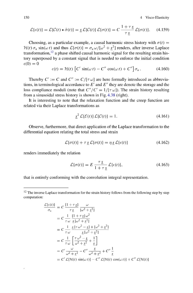
Choosing, as a particular example, a causal harmonic stress history with σ(t) =
H(t) σ a sin(ω t) and thus L{σ(t)} = σ a ω/[ω
2
+ s
2
] renders, after inverse Laplace
transformation,
12 a phase shifted causal harmonic signal for the resulting strain history superposed by a constant signal that is needed to enforce the initial condition
(0) = 0
(t) = H(t)
C
sin(ω t) − C
cos(ω t) + C
σ a .
(4.160)
Thereby C
:= C and C
:= C/[τ ω] are here formally introduced as abbreviations, in terminological accordance to E
and E
they are denote the storage and the
loss compliance moduli (note that C
/C
= 1/[τ ω]). The strain history resulting
from a sinusoidal stress history is shown in Fig. 4.38 (right).
It is interesting to note that the relaxation function and the creep function are
related via their Laplace transformations as
s
2
L{E(t)} L{C(t)} = 1.
(4.161)
Observe, furthermore, that direct application of the Laplace transformation to the
differential equation relating the total stress and strain
L{σ(t)} + τ s L{σ(t)} = η s L{(t)}
(4.162)
renders immediately the relation
L{σ(t)} = E
τ s
1 + τ s
L{(t)},
(4.163)
that is entirely conforming with the convolution integral representation.
12 The inverse Laplace transformation for the strain history follows from the following step by step
computation:
L{(t)}
σ a
= C
[1 + τ s]
τ s
ω
[ω 2 + s 2 ]
= C
1
τ ω
[1 + τ s] ω 2
s [ω 2 + s 2 ]
= C
1
τ ω
s [τ ω 2 − s] + [ω 2 + s 2 ]
s [ω 2 + s 2 ]
= C
1
τ ω
τ ω 2 − s
ω 2 + s 2 +
1
s
= C
ω
ω 2 + s 2 − C
s
ω 2 + s 2 + C
1
s
= C
L{H(t) sin(ω t)} − C
L{H(t) cos(ω t)} + C
L{H(t)}
.
4 Visco-Elasticity
L{(t)} = L{C(t) ) ˙
σ(t)} = s L{C(t)} L{σ(t)} = C
1 + τ s
τ s
L{σ(t)}. (4.159)
Choosing, as a particular example, a causal harmonic stress history with σ(t) =
H(t) σ a sin(ω t) and thus L{σ(t)} = σ a ω/[ω
2
+ s
2
] renders, after inverse Laplace
transformation,
12 a phase shifted causal harmonic signal for the resulting strain history superposed by a constant signal that is needed to enforce the initial condition
(0) = 0
(t) = H(t)
C
sin(ω t) − C
cos(ω t) + C
σ a .
(4.160)
Thereby C
:= C and C
:= C/[τ ω] are here formally introduced as abbreviations, in terminological accordance to E
and E
they are denote the storage and the
loss compliance moduli (note that C
/C
= 1/[τ ω]). The strain history resulting
from a sinusoidal stress history is shown in Fig. 4.38 (right).
It is interesting to note that the relaxation function and the creep function are
related via their Laplace transformations as
s
2
L{E(t)} L{C(t)} = 1.
(4.161)
Observe, furthermore, that direct application of the Laplace transformation to the
differential equation relating the total stress and strain
L{σ(t)} + τ s L{σ(t)} = η s L{(t)}
(4.162)
renders immediately the relation
L{σ(t)} = E
τ s
1 + τ s
L{(t)},
(4.163)
that is entirely conforming with the convolution integral representation.
12 The inverse Laplace transformation for the strain history follows from the following step by step
computation:
L{(t)}
σ a
= C
[1 + τ s]
τ s
ω
[ω 2 + s 2 ]
= C
1
τ ω
[1 + τ s] ω 2
s [ω 2 + s 2 ]
= C
1
τ ω
s [τ ω 2 − s] + [ω 2 + s 2 ]
s [ω 2 + s 2 ]
= C
1
τ ω
τ ω 2 − s
ω 2 + s 2 +
1
s
= C
ω
ω 2 + s 2 − C
s
ω 2 + s 2 + C
1
s
= C
L{H(t) sin(ω t)} − C
L{H(t) cos(ω t)} + C
L{H(t)}
.