

148
4 Visco-Elasticity
0
1
2
3
t
E(t)/E = H(t) e
−t/τ
τ
(t) 0 = H(t)
0
1
2
3
0
1
2
3
0
1
2
3
t
C(t)/C = H(t) [1 + t/τ ]
σ(t)/σ0 = H(t)
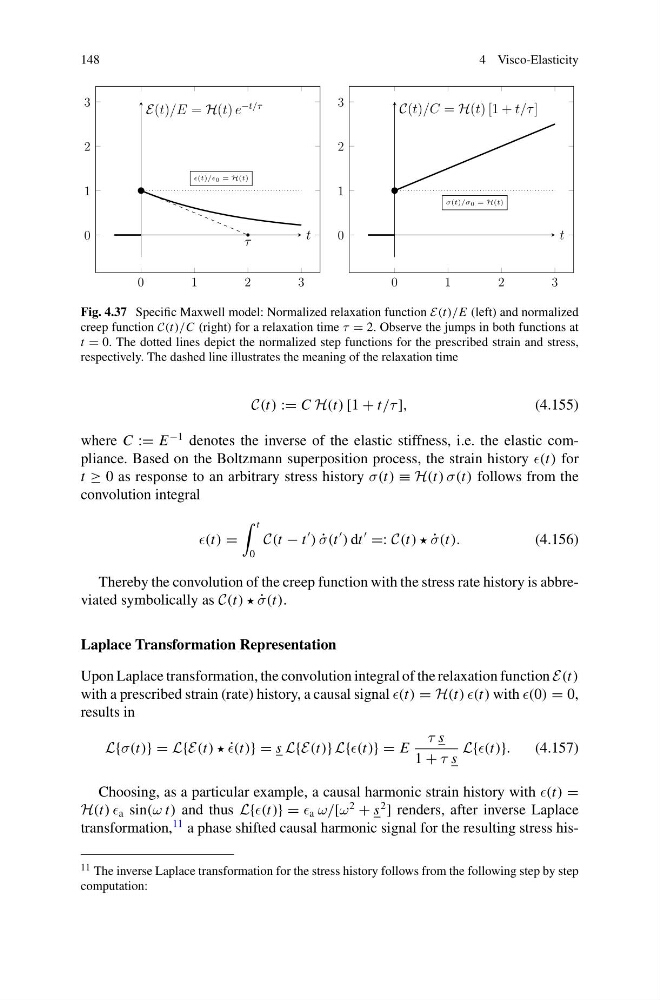
Fig. 4.37 Specific Maxwell model: Normalized relaxation function E(t)/E (left) and normalized
creep function C(t)/C (right) for a relaxation time τ = 2. Observe the jumps in both functions at
t = 0. The dotted lines depict the normalized step functions for the prescribed strain and stress,
respectively. The dashed line illustrates the meaning of the relaxation time
C(t) := C H(t) [1 + t/τ ],
(4.155)
where C := E
−1 denotes the inverse of the elastic stiffness, i.e. the elastic compliance. Based on the Boltzmann superposition process, the strain history for
t ≥ 0 as response to an arbitrary stress history σ(t) ≡ H(t) σ(t) follows from the
convolution integral
=
t
0
C(t − t
) ˙
σ(t
) dt
=: C(t) ) ˙
σ(t).
(4.156)
Thereby the convolution of the creep function with the stress rate history is abbreviated symbolically as C(t) ) ˙
σ(t).
Laplace Transformation Representation
Upon Laplace transformation, the convolution integral of the relaxation function E(t)
with a prescribed strain (rate) history, a causal signal = H(t) with = 0,
results in
L{σ(t)} = L{E(t) ) ˙
= s L{E(t)} L{ = E
τ s
1 + τ s
L{
(4.157)
Choosing, as a particular example, a causal harmonic strain history with =
H(t) a sin(ω t) and thus L{ = a ω/[ω
2
+ s
2
] renders, after inverse Laplace
transformation,
11 a phase shifted causal harmonic signal for the resulting stress his11 The inverse Laplace transformation for the stress history follows from the following step by step
computation:
4 Visco-Elasticity
0
1
2
3
t
E(t)/E = H(t) e
−t/τ
τ
(t) 0 = H(t)
0
1
2
3
0
1
2
3
0
1
2
3
t
C(t)/C = H(t) [1 + t/τ ]
σ(t)/σ0 = H(t)
Fig. 4.37 Specific Maxwell model: Normalized relaxation function E(t)/E (left) and normalized
creep function C(t)/C (right) for a relaxation time τ = 2. Observe the jumps in both functions at
t = 0. The dotted lines depict the normalized step functions for the prescribed strain and stress,
respectively. The dashed line illustrates the meaning of the relaxation time
C(t) := C H(t) [1 + t/τ ],
(4.155)
where C := E
−1 denotes the inverse of the elastic stiffness, i.e. the elastic compliance. Based on the Boltzmann superposition process, the strain history for
t ≥ 0 as response to an arbitrary stress history σ(t) ≡ H(t) σ(t) follows from the
convolution integral
=
t
0
C(t − t
) ˙
σ(t
) dt
=: C(t) ) ˙
σ(t).
(4.156)
Thereby the convolution of the creep function with the stress rate history is abbreviated symbolically as C(t) ) ˙
σ(t).
Laplace Transformation Representation
Upon Laplace transformation, the convolution integral of the relaxation function E(t)
with a prescribed strain (rate) history, a causal signal = H(t) with = 0,
results in
L{σ(t)} = L{E(t) ) ˙
= s L{E(t)} L{ = E
τ s
1 + τ s
L{
(4.157)
Choosing, as a particular example, a causal harmonic strain history with =
H(t) a sin(ω t) and thus L{ = a ω/[ω
2
+ s
2
] renders, after inverse Laplace
transformation,
11 a phase shifted causal harmonic signal for the resulting stress his11 The inverse Laplace transformation for the stress history follows from the following step by step
computation: