

140
4 Visco-Elasticity
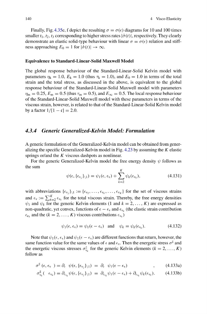
Finally, Fig. 4.35e, f depict the resulting σ = σ() diagrams for 10 and 100 times
smaller t 1 , t 2 , t 3 corresponding to higher stress rates | ˙
σ(t)|, respectively. They clearly
demonstrate an elastic solid-type behaviour with linear σ = σ() relation and stiffness approaching E 0 = 1 for | ˙
σ(t)| → ∞.
Equivalence to Standard-Linear-Solid Maxwell Model
The global response behaviour of the Standard-Linear-Solid Kelvin model with
parameters η k = 1.0, E k = 1.0 (thus τ k = 1.0), and E 0 = 1.0 in terms of the total
strain and the total stress, as discussed in the above, is equivalent to the global
response behaviour of the Standard-Linear-Solid Maxwell model with parameters
η m = 0.25, E m = 0.5 (thus τ m = 0.5), and E ∞ = 0.5. The local response behaviour
of the Standard-Linear-Solid Maxwell model with these parameters in terms of the
viscous strain, however, is related to that of the Standard-Linear-Solid Kelvin model
by a factor 1/[1 − c] = 2.0.
4.3.4 Generic Generalized-Kelvin Model: Formulation
A generic formulation of the Generalized-Kelvin model can be obtained from generalizing the specific Generalized-Kelvin model in Fig. 4.23 by assuming the K elastic
springs or/and the K viscous dashpots as nonlinear.
For the generic Generalized-Kelvin model the free energy density ψ follows as
the sum
ψ(, { v j } \1 ) = ψ 1 (, v ) +
K
k=2
ψ k ( v k ),
(4.131)
with abbreviations { v j } \1 := { v 2 , . . . , v k , . . . , v K } for the set of viscous strains
and v :=
K
k=2 v k for the total viscous strain. Thereby, the free energy densities
ψ 1 and ψ k for the generic Kelvin elements (1 and k = 2, . . . , K ) are expressed as
non-quadratic, yet convex, functions of − v and v k (the elastic strain contribution
e 1 and the (k = 2, . . . , K ) viscous contributions v k )
ψ 1 (, v ) = ψ 1 ( − v ) and ψ k = ψ k ( v k ).
(4.132)
Note that ψ 1 (, v ) and ψ 1 ( − v ) are different functions that return, however, the
same function value for the same values of and v . Then the energetic stress σ
and
the energetic viscous stresses σ
v k
for the generic Kelvin elements (k = 2, . . . , K )
follow as
σ
(, v ) = ∂ ψ(, { v j } \1 ) = ∂ ψ 1 ( − v )
,
(4.133a)
σ
v k
( v k ) = ∂ v k ψ(, { v j } \1 ) = ∂ v k ψ 1 ( − v ) + ∂ v k ψ k ( v k ).
(4.133b)
4 Visco-Elasticity
Finally, Fig. 4.35e, f depict the resulting σ = σ() diagrams for 10 and 100 times
smaller t 1 , t 2 , t 3 corresponding to higher stress rates | ˙
σ(t)|, respectively. They clearly
demonstrate an elastic solid-type behaviour with linear σ = σ() relation and stiffness approaching E 0 = 1 for | ˙
σ(t)| → ∞.
Equivalence to Standard-Linear-Solid Maxwell Model
The global response behaviour of the Standard-Linear-Solid Kelvin model with
parameters η k = 1.0, E k = 1.0 (thus τ k = 1.0), and E 0 = 1.0 in terms of the total
strain and the total stress, as discussed in the above, is equivalent to the global
response behaviour of the Standard-Linear-Solid Maxwell model with parameters
η m = 0.25, E m = 0.5 (thus τ m = 0.5), and E ∞ = 0.5. The local response behaviour
of the Standard-Linear-Solid Maxwell model with these parameters in terms of the
viscous strain, however, is related to that of the Standard-Linear-Solid Kelvin model
by a factor 1/[1 − c] = 2.0.
4.3.4 Generic Generalized-Kelvin Model: Formulation
A generic formulation of the Generalized-Kelvin model can be obtained from generalizing the specific Generalized-Kelvin model in Fig. 4.23 by assuming the K elastic
springs or/and the K viscous dashpots as nonlinear.
For the generic Generalized-Kelvin model the free energy density ψ follows as
the sum
ψ(, { v j } \1 ) = ψ 1 (, v ) +
K
k=2
ψ k ( v k ),
(4.131)
with abbreviations { v j } \1 := { v 2 , . . . , v k , . . . , v K } for the set of viscous strains
and v :=
K
k=2 v k for the total viscous strain. Thereby, the free energy densities
ψ 1 and ψ k for the generic Kelvin elements (1 and k = 2, . . . , K ) are expressed as
non-quadratic, yet convex, functions of − v and v k (the elastic strain contribution
e 1 and the (k = 2, . . . , K ) viscous contributions v k )
ψ 1 (, v ) = ψ 1 ( − v ) and ψ k = ψ k ( v k ).
(4.132)
Note that ψ 1 (, v ) and ψ 1 ( − v ) are different functions that return, however, the
same function value for the same values of and v . Then the energetic stress σ
and
the energetic viscous stresses σ
v k
for the generic Kelvin elements (k = 2, . . . , K )
follow as
σ
(, v ) = ∂ ψ(, { v j } \1 ) = ∂ ψ 1 ( − v )
,
(4.133a)
σ
v k
( v k ) = ∂ v k ψ(, { v j } \1 ) = ∂ v k ψ 1 ( − v ) + ∂ v k ψ k ( v k ).
(4.133b)