

188
Appendix I
Correspondingly:
(f
2 ) ω =
¯
hα (ω)
| α(ω) | 2 coth
¯
hω
2kT
(I.6)
The mean square of the fluctuating quantity is:
< x
2 >=
1
π
∞
0
(x
2 ) ω dω =
¯
h
π
∞
0
α
(ω) coth
¯
hω
2kT
dω
(I.7)
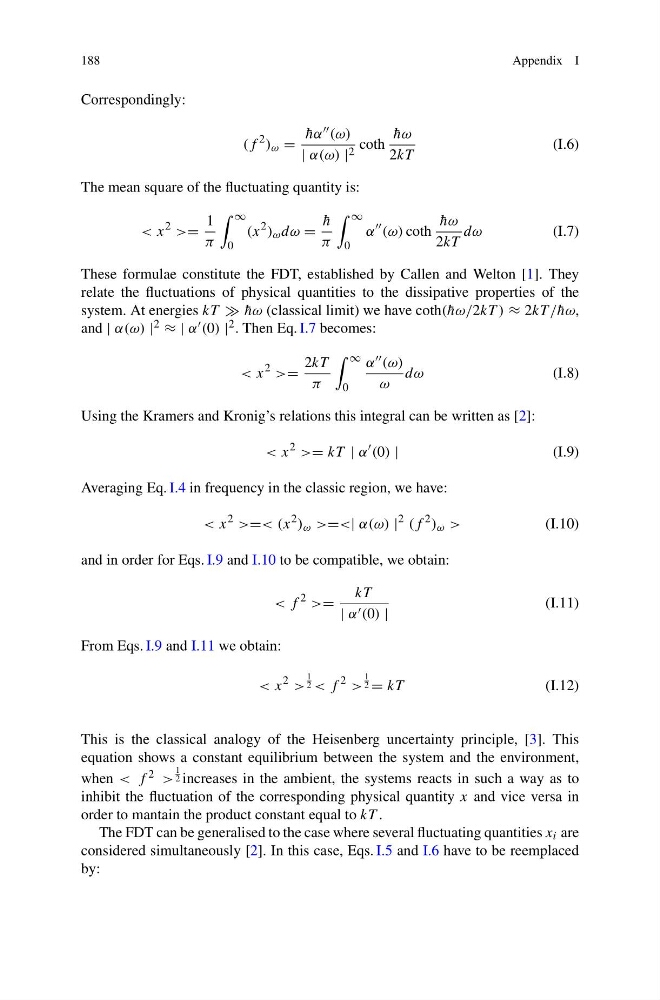
These formulae constitute the FDT, established by Callen and Welton [1]. They
relate the fluctuations of physical quantities to the dissipative properties of the
system. At energies kT ¯
hω (classical limit) we have coth( ¯
hω/2kT ) ≈ 2kT / ¯
hω,
and | α(ω) | 2 ≈ | α (0) | 2 . Then Eq. I.7 becomes:
< x
2 >=
2kT
π
∞
0
α (ω)
ω
dω
(I.8)
Using the Kramers and Kronig’s relations this integral can be written as [2]:
< x
2 >= kT | α
(0) |
(I.9)
Averaging Eq. I.4 in frequency in the classic region, we have:
< x
2 >=< (x
2 ) ω >=<| α(ω) |
2 (f
2 ) ω >
(I.10)
and in order for Eqs. I.9 and I.10 to be compatible, we obtain:
< f
2 >=
kT
| α (0) |
(I.11)
From Eqs. I.9 and I.11 we obtain:
< x
2 >
1
2 < f
2 >
1
2 = kT
(I.12)
This is the classical analogy of the Heisenberg uncertainty principle, [3]. This
equation shows a constant equilibrium between the system and the environment,
when < f 2 >
1
2 increases in the ambient, the systems reacts in such a way as to
inhibit the fluctuation of the corresponding physical quantity x and vice versa in
order to mantain the product constant equal to kT .
The FDT can be generalised to the case where several fluctuating quantities x i are
considered simultaneously [2]. In this case, Eqs. I.5 and I.6 have to be reemplaced
by:
Appendix I
Correspondingly:
(f
2 ) ω =
¯
hα (ω)
| α(ω) | 2 coth
¯
hω
2kT
(I.6)
The mean square of the fluctuating quantity is:
< x
2 >=
1
π
∞
0
(x
2 ) ω dω =
¯
h
π
∞
0
α
(ω) coth
¯
hω
2kT
dω
(I.7)
These formulae constitute the FDT, established by Callen and Welton [1]. They
relate the fluctuations of physical quantities to the dissipative properties of the
system. At energies kT ¯
hω (classical limit) we have coth( ¯
hω/2kT ) ≈ 2kT / ¯
hω,
and | α(ω) | 2 ≈ | α (0) | 2 . Then Eq. I.7 becomes:
< x
2 >=
2kT
π
∞
0
α (ω)
ω
dω
(I.8)
Using the Kramers and Kronig’s relations this integral can be written as [2]:
< x
2 >= kT | α
(0) |
(I.9)
Averaging Eq. I.4 in frequency in the classic region, we have:
< x
2 >=< (x
2 ) ω >=<| α(ω) |
2 (f
2 ) ω >
(I.10)
and in order for Eqs. I.9 and I.10 to be compatible, we obtain:
< f
2 >=
kT
| α (0) |
(I.11)
From Eqs. I.9 and I.11 we obtain:
< x
2 >
1
2 < f
2 >
1
2 = kT
(I.12)
This is the classical analogy of the Heisenberg uncertainty principle, [3]. This
equation shows a constant equilibrium between the system and the environment,
when < f 2 >
1
2 increases in the ambient, the systems reacts in such a way as to
inhibit the fluctuation of the corresponding physical quantity x and vice versa in
order to mantain the product constant equal to kT .
The FDT can be generalised to the case where several fluctuating quantities x i are
considered simultaneously [2]. In this case, Eqs. I.5 and I.6 have to be reemplaced
by: