

3.5 Jet Substructure Tagging
85
Top quark tagging efficiency
0
0.5
1
Background rejection
1
10
2
10
3
10
SD (C/A 0.2 subjets)
SD (C/A 0.2 subjets) WP
HEPTopTagger (C/A 1.5)
12
d
trimmed mass
)
23
d
Tagger V (scan
)
32
τ
W' Tagger (scan
23
d
32
τ
Tagger I
Tagger II
Tagger III
Tagger IV
Tagger V
W' Top Tagger
ATLAS
= 8 TeV
s
Simulation
< 400 GeV
T
350 GeV < p
S
ε
0
0.2
0.4
0.6
0.8
1
B
ε
4
−
10
3
−
10
2
−
10
1
−
10
CMS
Simulation Preliminary
13 TeV
| < 1.5
η
< 1000 GeV, |
T
800 < p
R(top,parton) < 0.6
Δ
η
and
T
flat p
CMSTT min. m
CMSTT top m
Filtered (r=0.2, n=3) m
Rec
HTT V2 f
HTT V2 m
=0.5) m
cut
Pruned (z=0.1, r
Q-jet volatility
=0) m
β
Softdrop (z=0.1,
=1) m
β
Softdrop (z=0.2,
Trimmed (r=0.2, f=0.03) m
2
τ
/
3
τ
Ungroomed
) (R=0.2)
χ
log(
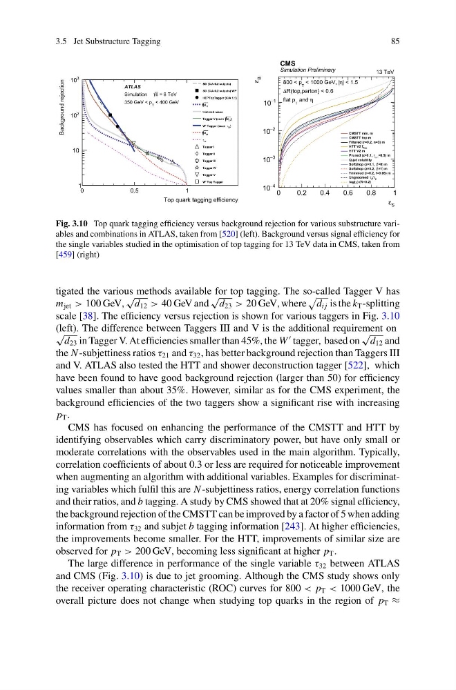
Fig. 3.10 Top quark tagging efficiency versus background rejection for various substructure variables and combinations in ATLAS, taken from [520] (left). Background versus signal efficiency for
the single variables studied in the optimisation of top tagging for 13 TeV data in CMS, taken from
[459] (right)
tigated the various methods available for top tagging. The so-called Tagger V has
m jet > 100 GeV,
√
d 12 > 40 GeV and
√
d 23 > 20 GeV, where
d i j is the k T -splitting
scale [38]. The efficiency versus rejection is shown for various taggers in Fig. 3.10
(left). The difference between Taggers III and V is the additional requirement on
√
d 23 in Tagger V. At efficiencies smaller than 45%, the W
tagger, based on
√
d 12 and
the N -subjettiness ratios τ 21 and τ 32 , has better background rejection than Taggers III
and V. ATLAS also tested the HTT and shower deconstruction tagger [522], which
have been found to have good background rejection (larger than 50) for efficiency
values smaller than about 35%. However, similar as for the CMS experiment, the
background efficiencies of the two taggers show a significant rise with increasing
p T .
CMS has focused on enhancing the performance of the CMSTT and HTT by
identifying observables which carry discriminatory power, but have only small or
moderate correlations with the observables used in the main algorithm. Typically,
correlation coefficients of about 0.3 or less are required for noticeable improvement
when augmenting an algorithm with additional variables. Examples for discriminating variables which fulfil this are N -subjettiness ratios, energy correlation functions
and their ratios, and b tagging. A study by CMS showed that at 20% signal efficiency,
the background rejection of the CMSTT can be improved by a factor of 5 when adding
information from τ 32 and subjet b tagging information [243]. At higher efficiencies,
the improvements become smaller. For the HTT, improvements of similar size are
observed for p T > 200 GeV, becoming less significant at higher p T .
The large difference in performance of the single variable τ 32 between ATLAS
and CMS (Fig. 3.10) is due to jet grooming. Although the CMS study shows only
the receiver operating characteristic (ROC) curves for 800 < p T < 1000 GeV, the
overall picture does not change when studying top quarks in the region of p T ≈
85
Top quark tagging efficiency
0
0.5
1
Background rejection
1
10
2
10
3
10
SD (C/A 0.2 subjets)
SD (C/A 0.2 subjets) WP
HEPTopTagger (C/A 1.5)
12
d
trimmed mass
)
23
d
Tagger V (scan
)
32
τ
W' Tagger (scan
23
d
32
τ
Tagger I
Tagger II
Tagger III
Tagger IV
Tagger V
W' Top Tagger
ATLAS
= 8 TeV
s
Simulation
< 400 GeV
T
350 GeV < p
S
ε
0
0.2
0.4
0.6
0.8
1
B
ε
4
−
10
3
−
10
2
−
10
1
−
10
CMS
Simulation Preliminary
13 TeV
| < 1.5
η
< 1000 GeV, |
T
800 < p
R(top,parton) < 0.6
Δ
η
and
T
flat p
CMSTT min. m
CMSTT top m
Filtered (r=0.2, n=3) m
Rec
HTT V2 f
HTT V2 m
=0.5) m
cut
Pruned (z=0.1, r
Q-jet volatility
=0) m
β
Softdrop (z=0.1,
=1) m
β
Softdrop (z=0.2,
Trimmed (r=0.2, f=0.03) m
2
τ
/
3
τ
Ungroomed
) (R=0.2)
χ
log(
Fig. 3.10 Top quark tagging efficiency versus background rejection for various substructure variables and combinations in ATLAS, taken from [520] (left). Background versus signal efficiency for
the single variables studied in the optimisation of top tagging for 13 TeV data in CMS, taken from
[459] (right)
tigated the various methods available for top tagging. The so-called Tagger V has
m jet > 100 GeV,
√
d 12 > 40 GeV and
√
d 23 > 20 GeV, where
d i j is the k T -splitting
scale [38]. The efficiency versus rejection is shown for various taggers in Fig. 3.10
(left). The difference between Taggers III and V is the additional requirement on
√
d 23 in Tagger V. At efficiencies smaller than 45%, the W
tagger, based on
√
d 12 and
the N -subjettiness ratios τ 21 and τ 32 , has better background rejection than Taggers III
and V. ATLAS also tested the HTT and shower deconstruction tagger [522], which
have been found to have good background rejection (larger than 50) for efficiency
values smaller than about 35%. However, similar as for the CMS experiment, the
background efficiencies of the two taggers show a significant rise with increasing
p T .
CMS has focused on enhancing the performance of the CMSTT and HTT by
identifying observables which carry discriminatory power, but have only small or
moderate correlations with the observables used in the main algorithm. Typically,
correlation coefficients of about 0.3 or less are required for noticeable improvement
when augmenting an algorithm with additional variables. Examples for discriminating variables which fulfil this are N -subjettiness ratios, energy correlation functions
and their ratios, and b tagging. A study by CMS showed that at 20% signal efficiency,
the background rejection of the CMSTT can be improved by a factor of 5 when adding
information from τ 32 and subjet b tagging information [243]. At higher efficiencies,
the improvements become smaller. For the HTT, improvements of similar size are
observed for p T > 200 GeV, becoming less significant at higher p T .
The large difference in performance of the single variable τ 32 between ATLAS
and CMS (Fig. 3.10) is due to jet grooming. Although the CMS study shows only
the receiver operating characteristic (ROC) curves for 800 < p T < 1000 GeV, the
overall picture does not change when studying top quarks in the region of p T ≈