

2.4 Identifying Particle Decays with Jet Substructure
43
φ
3
−
2
−
1
−
0
1
2
3
η
3
−
2
−
1
−
0
1
2
3
Event 1
clustered with CA
φ
3
−
2
−
1
−
0
1
2
3
η
3
−
2
−
1
−
0
1
2
3
HOTVR
Event 1
clustered with HOTVR
φ
3
−
2
−
1
−
0
1
2
3
η
3
−
2
−
1
−
0
1
2
3
Event 2
clustered with CA
φ
3
−
2
−
1
−
0
1
2
3
η
3
−
2
−
1
−
0
1
2
3
HOTVR
Event 2
clustered with HOTVR
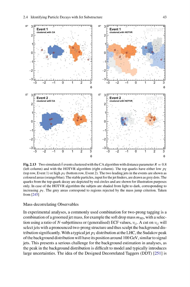
Fig. 2.13 Two simulated tt events clustered with the CA algorithm with distance parameter R = 0.8
(left column) and with the HOTVR algorithm (right column). The top quarks have either low p T
(top row, Event 1) or high p T (bottom row, Event 2). The two leading jets in the events are shown as
coloured areas (orange/blue). The stable particles, input for the jet finders, are drawn as grey dots. The
quarks from the top quark decay are depicted by red circles and are shown for illustration purposes
only. In case of the HOTVR algorithm the subjets are shaded from light to dark, corresponding to
increasing p T . The grey areas correspond to regions rejected by the mass jump criterion. Taken
from [245]
Mass-decorrelating Observables
In experimental analyses, a commonly used combination for two-prong tagging is a
combination of a groomed jet mass, for example the soft drop mass m SD , with a selection using a ratio of N -subjettiness or (generalised) ECF values, ν i j . A cut on ν i j will
select jets with a pronounced two-prong structure and thus sculpt the background distribution significantly. With a typical jet p T distribution at the LHC, the Sudakov peak
of the background distribution will have its position around 100 GeV, similar to signal
jets. This presents a serious challenge for the background estimation in analyses, as
the peak in the background distribution is difficult to model and typically introduces
large uncertainties. The idea of the Designed Decorrelated Taggers (DDT) [251] is
43
φ
3
−
2
−
1
−
0
1
2
3
η
3
−
2
−
1
−
0
1
2
3
Event 1
clustered with CA
φ
3
−
2
−
1
−
0
1
2
3
η
3
−
2
−
1
−
0
1
2
3
HOTVR
Event 1
clustered with HOTVR
φ
3
−
2
−
1
−
0
1
2
3
η
3
−
2
−
1
−
0
1
2
3
Event 2
clustered with CA
φ
3
−
2
−
1
−
0
1
2
3
η
3
−
2
−
1
−
0
1
2
3
HOTVR
Event 2
clustered with HOTVR
Fig. 2.13 Two simulated tt events clustered with the CA algorithm with distance parameter R = 0.8
(left column) and with the HOTVR algorithm (right column). The top quarks have either low p T
(top row, Event 1) or high p T (bottom row, Event 2). The two leading jets in the events are shown as
coloured areas (orange/blue). The stable particles, input for the jet finders, are drawn as grey dots. The
quarks from the top quark decay are depicted by red circles and are shown for illustration purposes
only. In case of the HOTVR algorithm the subjets are shaded from light to dark, corresponding to
increasing p T . The grey areas correspond to regions rejected by the mass jump criterion. Taken
from [245]
Mass-decorrelating Observables
In experimental analyses, a commonly used combination for two-prong tagging is a
combination of a groomed jet mass, for example the soft drop mass m SD , with a selection using a ratio of N -subjettiness or (generalised) ECF values, ν i j . A cut on ν i j will
select jets with a pronounced two-prong structure and thus sculpt the background distribution significantly. With a typical jet p T distribution at the LHC, the Sudakov peak
of the background distribution will have its position around 100 GeV, similar to signal
jets. This presents a serious challenge for the background estimation in analyses, as
the peak in the background distribution is difficult to model and typically introduces
large uncertainties. The idea of the Designed Decorrelated Taggers (DDT) [251] is