

4.3 LSTM
67
|h(t)
. . .
|c(t − 1)
+
|c(t)
. . .
g f
g i
tanh
tanh
. . .
|h(t − 1)
⊕
J
f
x ⊕J
f
h
J
i
x ⊕J
i
h
Jx⊕Jh
J
o
x ⊕J
o
h
g o
|h(t)
. . .
|x(t)
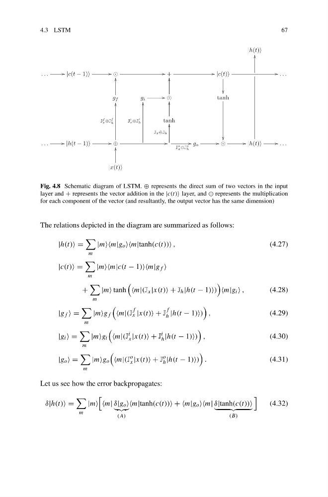
Fig. 4.8 Schematic diagram of LSTM. ⊕ represents the direct sum of two vectors in the input
layer and + represents the vector addition in the |c(t) layer, and represents the multiplication
for each component of the vector (and resultantly, the output vector has the same dimension)
The relations depicted in the diagram are summarized as follows:
|h(t) =
m
|m o ,
(4.27)
|c(t) =
m
|m − 1) f
+
m
|m tanh
x |x(t) + J h |h(t − 1)
i ,
(4.28)
|g f =
m
|m f
f
x |x(t) + J
f
h |h(t − 1)
,
(4.29)
|g i =
m
|m i
i
x |x(t) + J
i
h |h(t − 1)
,
(4.30)
|g o =
m
|m o
o
x |x(t) + J
o
h |h(t − 1)
.
(4.31)
Let us see how the error backpropagates:
δ|h(t) =
m
|m
δ|g o
(A)
+ +m|g o δ|tanh(c(t))
(B)
(4.32)
67
|h(t)
. . .
|c(t − 1)
+
|c(t)
. . .
g f
g i
tanh
tanh
. . .
|h(t − 1)
⊕
J
f
x ⊕J
f
h
J
i
x ⊕J
i
h
Jx⊕Jh
J
o
x ⊕J
o
h
g o
|h(t)
. . .
|x(t)
Fig. 4.8 Schematic diagram of LSTM. ⊕ represents the direct sum of two vectors in the input
layer and + represents the vector addition in the |c(t) layer, and represents the multiplication
for each component of the vector (and resultantly, the output vector has the same dimension)
The relations depicted in the diagram are summarized as follows:
|h(t) =
m
|m o ,
(4.27)
|c(t) =
m
|m − 1) f
+
m
|m tanh
x |x(t) + J h |h(t − 1)
i ,
(4.28)
|g f =
m
|m f
f
x |x(t) + J
f
h |h(t − 1)
,
(4.29)
|g i =
m
|m i
i
x |x(t) + J
i
h |h(t − 1)
,
(4.30)
|g o =
m
|m o
o
x |x(t) + J
o
h |h(t − 1)
.
(4.31)
Let us see how the error backpropagates:
δ|h(t) =
m
|m
δ|g o
(A)
+ +m|g o δ|tanh(c(t))
(B)
(4.32)