

4.2 Recurrent Neural Network and Backpropagation
63
|h(t)
. . .
|h(t − 1)
⊕ J h ⊕Jx
σ •
|h(t)
. . .
|x(t)
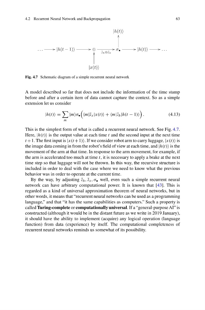
Fig. 4.7 Schematic diagram of a simple recurrent neural network
A model described so far that does not include the information of the time stamp
before and after a certain item of data cannot capture the context. So as a simple
extension let us consider
|h(t) =
m
|mσ •
m|J x |x(t) + +m|J h |h(t − 1)
.
(4.13)
This is the simplest form of what is called a recurrent neural network. See Fig. 4.7.
Here, |h(t) is the output value at each time t and the second input at the next time
t +1. The first input is |x(t +1). If we consider robot arm to carry luggage, |x(t) is
the image data coming in from the robot’s field of view at each time, and |h(t) is the
movement of the arm at that time. In response to the arm movement, for example, if
the arm is accelerated too much at time t, it is necessary to apply a brake at the next
time step so that luggage will not be thrown. In this way, the recursive structure is
included in order to deal with the case where we need to know what the previous
behavior was in order to operate at the current time.
By the way, by adjusting J h , J x , σ • well, even such a simple recurrent neural
network can have arbitrary computational power. It is known that [43]. This is
regarded as a kind of universal approximation theorem of neural networks, but in
other words, it means that “recurrent neural networks can be used as a programming
language,” and that “it has the same capabilities as computers.” Such a property is
called Turing-complete or computationally universal. If a “general-purpose AI” is
constructed (although it would be in the distant future as we write in 2019 January),
it should have the ability to implement (acquire) any logical operation (language
function) from data (experience) by itself. The computational completeness of
recurrent neural networks reminds us somewhat of its possibility.
63
|h(t)
. . .
|h(t − 1)
⊕ J h ⊕Jx
σ •
|h(t)
. . .
|x(t)
Fig. 4.7 Schematic diagram of a simple recurrent neural network
A model described so far that does not include the information of the time stamp
before and after a certain item of data cannot capture the context. So as a simple
extension let us consider
|h(t) =
m
|mσ •
m|J x |x(t) + +m|J h |h(t − 1)
.
(4.13)
This is the simplest form of what is called a recurrent neural network. See Fig. 4.7.
Here, |h(t) is the output value at each time t and the second input at the next time
t +1. The first input is |x(t +1). If we consider robot arm to carry luggage, |x(t) is
the image data coming in from the robot’s field of view at each time, and |h(t) is the
movement of the arm at that time. In response to the arm movement, for example, if
the arm is accelerated too much at time t, it is necessary to apply a brake at the next
time step so that luggage will not be thrown. In this way, the recursive structure is
included in order to deal with the case where we need to know what the previous
behavior was in order to operate at the current time.
By the way, by adjusting J h , J x , σ • well, even such a simple recurrent neural
network can have arbitrary computational power. It is known that [43]. This is
regarded as a kind of universal approximation theorem of neural networks, but in
other words, it means that “recurrent neural networks can be used as a programming
language,” and that “it has the same capabilities as computers.” Such a property is
called Turing-complete or computationally universal. If a “general-purpose AI” is
constructed (although it would be in the distant future as we write in 2019 January),
it should have the ability to implement (acquire) any logical operation (language
function) from data (experience) by itself. The computational completeness of
recurrent neural networks reminds us somewhat of its possibility.