

58
4 Advanced Neural Networks
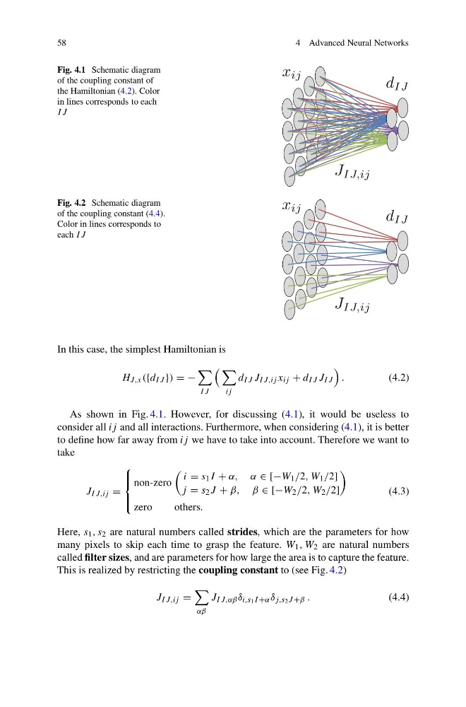
Fig. 4.1 Schematic diagram
of the coupling constant of
the Hamiltonian (4.2). Color
in lines corresponds to each
IJ
x ij
d IJ
J IJ,ij
Fig. 4.2 Schematic diagram
of the coupling constant (4.4).
Color in lines corresponds to
each IJ
x ij
d IJ
J IJ,ij
In this case, the simplest Hamiltonian is
H J,x ({d I J }) = −
I J
ij
d I J J I J,ij x ij + d I J J I J
.
(4.2)
As shown in Fig. 4.1. However, for discussing (4.1), it would be useless to
consider all ij and all interactions. Furthermore, when considering (4.1), it is better
to define how far away from ij we have to take into account. Therefore we want to
take
J I J,ij =
⎧
⎪ ⎨
⎪ ⎩
non-zero
i = s 1 I + α, α ∈ [−W 1 /2, W 1 /2]
j = s 2 J + β, β ∈ [−W 2 /2, W 2 /2]
zero
others.
(4.3)
Here, s 1 , s 2 are natural numbers called strides, which are the parameters for how
many pixels to skip each time to grasp the feature. W 1 , W 2 are natural numbers
called filter sizes, and are parameters for how large the area is to capture the feature.
This is realized by restricting the coupling constant to (see Fig. 4.2)
J I J,ij =
αβ
J I J,αβ δ i,s 1 I +α δ j,s 2 J +β .
(4.4)
4 Advanced Neural Networks
Fig. 4.1 Schematic diagram
of the coupling constant of
the Hamiltonian (4.2). Color
in lines corresponds to each
IJ
x ij
d IJ
J IJ,ij
Fig. 4.2 Schematic diagram
of the coupling constant (4.4).
Color in lines corresponds to
each IJ
x ij
d IJ
J IJ,ij
In this case, the simplest Hamiltonian is
H J,x ({d I J }) = −
I J
ij
d I J J I J,ij x ij + d I J J I J
.
(4.2)
As shown in Fig. 4.1. However, for discussing (4.1), it would be useless to
consider all ij and all interactions. Furthermore, when considering (4.1), it is better
to define how far away from ij we have to take into account. Therefore we want to
take
J I J,ij =
⎧
⎪ ⎨
⎪ ⎩
non-zero
i = s 1 I + α, α ∈ [−W 1 /2, W 1 /2]
j = s 2 J + β, β ∈ [−W 2 /2, W 2 /2]
zero
others.
(4.3)
Here, s 1 , s 2 are natural numbers called strides, which are the parameters for how
many pixels to skip each time to grasp the feature. W 1 , W 2 are natural numbers
called filter sizes, and are parameters for how large the area is to capture the feature.
This is realized by restricting the coupling constant to (see Fig. 4.2)
J I J,ij =
αβ
J I J,αβ δ i,s 1 I +α δ j,s 2 J +β .
(4.4)