

3.1 Error Function from Statistical Mechanics
39
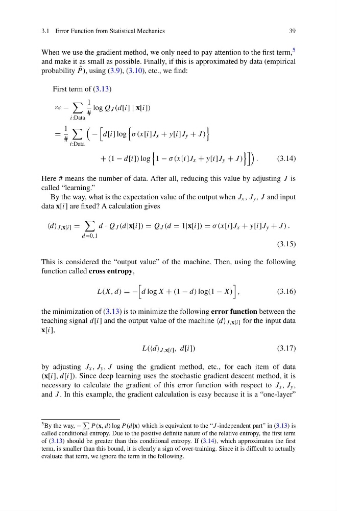
When we use the gradient method, we only need to pay attention to the first term, 5
and make it as small as possible. Finally, if this is approximated by data (empirical
probability ˆ
P ), using (3.9), (3.10), etc., we find:
First term of (3.13)
≈ −
i:Data
1
#
log Q J (d[i] | x[i])
=
1
#
i:Data
−
d[i] log
σ (x[i]J x + y[i]J y + J )
+ (1 − d[i]) log
1 − σ (x[i]J x + y[i]J y + J )
.
(3.14)
Here # means the number of data. After all, reducing this value by adjusting J is
called “learning.”
By the way, what is the expectation value of the output when J x , J y , J and input
data x[i] are fixed? A calculation gives
J,x[i] =
d=0,1
d · Q J (d|x[i]) = Q J (d = 1|x[i]) = σ (x[i]J x + y[i]J y + J ) .
(3.15)
This is considered the “output value” of the machine. Then, using the following
function called cross entropy,
L(X, d) = −
d log X + (1 − d) log(1 − X)
,
(3.16)
the minimization of (3.13) is to minimize the following error function between the
teaching signal d[i] and the output value of the machine J,x[i] for the input data
x[i],
L( J,x[i] , d[i])
(3.17)
by adjusting J x , J y , J using the gradient method, etc., for each item of data
(x[i], d[i]). Since deep learning uses the stochastic gradient descent method, it is
necessary to calculate the gradient of this error function with respect to J x , J y ,
and J . In this example, the gradient calculation is easy because it is a “one-layer”
5 By the way, −
P (x, d) log P (d|x) which is equivalent to the “J -independent part” in (3.13) is
called conditional entropy. Due to the positive definite nature of the relative entropy, the first term
of (3.13) should be greater than this conditional entropy. If (3.14), which approximates the first
term, is smaller than this bound, it is clearly a sign of over-training. Since it is difficult to actually
evaluate that term, we ignore the term in the following.
39
When we use the gradient method, we only need to pay attention to the first term, 5
and make it as small as possible. Finally, if this is approximated by data (empirical
probability ˆ
P ), using (3.9), (3.10), etc., we find:
First term of (3.13)
≈ −
i:Data
1
#
log Q J (d[i] | x[i])
=
1
#
i:Data
−
d[i] log
σ (x[i]J x + y[i]J y + J )
+ (1 − d[i]) log
1 − σ (x[i]J x + y[i]J y + J )
.
(3.14)
Here # means the number of data. After all, reducing this value by adjusting J is
called “learning.”
By the way, what is the expectation value of the output when J x , J y , J and input
data x[i] are fixed? A calculation gives
J,x[i] =
d=0,1
d · Q J (d|x[i]) = Q J (d = 1|x[i]) = σ (x[i]J x + y[i]J y + J ) .
(3.15)
This is considered the “output value” of the machine. Then, using the following
function called cross entropy,
L(X, d) = −
d log X + (1 − d) log(1 − X)
,
(3.16)
the minimization of (3.13) is to minimize the following error function between the
teaching signal d[i] and the output value of the machine J,x[i] for the input data
x[i],
L( J,x[i] , d[i])
(3.17)
by adjusting J x , J y , J using the gradient method, etc., for each item of data
(x[i], d[i]). Since deep learning uses the stochastic gradient descent method, it is
necessary to calculate the gradient of this error function with respect to J x , J y ,
and J . In this example, the gradient calculation is easy because it is a “one-layer”
5 By the way, −
P (x, d) log P (d|x) which is equivalent to the “J -independent part” in (3.13) is
called conditional entropy. Due to the positive definite nature of the relative entropy, the first term
of (3.13) should be greater than this conditional entropy. If (3.14), which approximates the first
term, is smaller than this bound, it is clearly a sign of over-training. Since it is difficult to actually
evaluate that term, we ignore the term in the following.