

36
3 Basics of Neural Networks
x
y
J x
J y
d
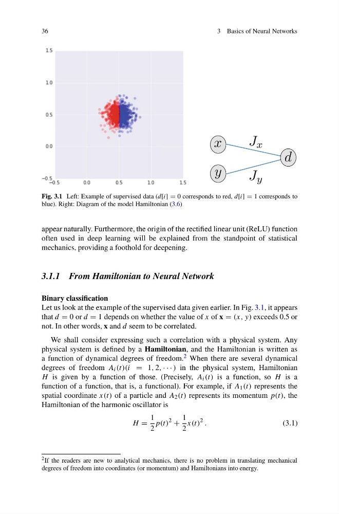
Fig. 3.1 Left: Example of supervised data (d[i] = 0 corresponds to red, d[i] = 1 corresponds to
blue). Right: Diagram of the model Hamiltonian (3.6)
appear naturally. Furthermore, the origin of the rectified linear unit (ReLU) function
often used in deep learning will be explained from the standpoint of statistical
mechanics, providing a foothold for deepening.
3.1.1 From Hamiltonian to Neural Network
Binary classification
Let us look at the example of the supervised data given earlier. In Fig. 3.1, it appears
that d = 0 or d = 1 depends on whether the value of x of x = (x, y) exceeds 0.5 or
not. In other words, x and d seem to be correlated.
We shall consider expressing such a correlation with a physical system. Any
physical system is defined by a Hamiltonian, and the Hamiltonian is written as
a function of dynamical degrees of freedom. 2 When there are several dynamical
degrees of freedom A i (t)(i = 1, 2, · · · ) in the physical system, Hamiltonian
H is given by a function of those. (Precisely, A i (t) is a function, so H is a
function of a function, that is, a functional). For example, if A 1 (t) represents the
spatial coordinate x(t) of a particle and A 2 (t) represents its momentum p(t), the
Hamiltonian of the harmonic oscillator is
H =
1
2
p(t)
2
+
1
2
x(t)
2 .
(3.1)
2 If the readers are new to analytical mechanics, there is no problem in translating mechanical
degrees of freedom into coordinates (or momentum) and Hamiltonians into energy.
3 Basics of Neural Networks
x
y
J x
J y
d
Fig. 3.1 Left: Example of supervised data (d[i] = 0 corresponds to red, d[i] = 1 corresponds to
blue). Right: Diagram of the model Hamiltonian (3.6)
appear naturally. Furthermore, the origin of the rectified linear unit (ReLU) function
often used in deep learning will be explained from the standpoint of statistical
mechanics, providing a foothold for deepening.
3.1.1 From Hamiltonian to Neural Network
Binary classification
Let us look at the example of the supervised data given earlier. In Fig. 3.1, it appears
that d = 0 or d = 1 depends on whether the value of x of x = (x, y) exceeds 0.5 or
not. In other words, x and d seem to be correlated.
We shall consider expressing such a correlation with a physical system. Any
physical system is defined by a Hamiltonian, and the Hamiltonian is written as
a function of dynamical degrees of freedom. 2 When there are several dynamical
degrees of freedom A i (t)(i = 1, 2, · · · ) in the physical system, Hamiltonian
H is given by a function of those. (Precisely, A i (t) is a function, so H is a
function of a function, that is, a functional). For example, if A 1 (t) represents the
spatial coordinate x(t) of a particle and A 2 (t) represents its momentum p(t), the
Hamiltonian of the harmonic oscillator is
H =
1
2
p(t)
2
+
1
2
x(t)
2 .
(3.1)
2 If the readers are new to analytical mechanics, there is no problem in translating mechanical
degrees of freedom into coordinates (or momentum) and Hamiltonians into energy.