

26
2 Introduction to Machine Learning
after setting an appropriate initial value J t =0 . This is called the gradient descent
method. 15 Here is a small positive real number. Then, for a change of J as δJ =
J t +1 − J t , the change of D KL is
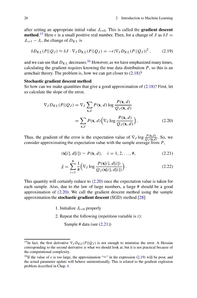
δD KL (P ||Q J ) ≈ δJ · ∇ J D KL (P ||Q J ) = −|∇ J D KL (P ||Q J )|
2 ,
(2.19)
and we can see that D KL decreases. 16 However, as we have emphasized many times,
calculating the gradient requires knowing the true data distribution P , so this is an
armchair theory. The problem is, how we can get closer to (2.18)?
Stochastic gradient descent method
So how can we make quantities that give a good approximation of (2.18)? First, let
us calculate the slope of the error,
∇ J D KL (P ||Q J ) = ∇ J
x,d
P (x, d) log
P (x, d)
Q J (x, d)
=
x,d
P (x, d)
∇ J log
P (x, d)
Q J (x, d)
.
(2.20)
Thus, the gradient of the error is the expectation value of ∇ J log
P (x,d)
Q J (x,d) . So, we
consider approximating the expectation value with the sample average from P ,
(x[i], d[i]) ∼ P (x, d), i = 1, 2, . . . , #,
(2.21)
ˆ
g =
#
i=1
1
#
∇ J log
P (x[i], d[i])
Q J (x[i], d[i])
.
(2.22)
This quantity will certainly reduce to (2.20) once the expectation value is taken for
each sample. Also, due to the law of large numbers, a large # should be a good
approximation of (2.20). We call the gradient descent method using the sample
approximation the stochastic gradient descent (SGD) method [28]:
1. Initialize J t =0 properly
2. Repeat the following (repetition variable is t):
Sample # data (see (2.21))
15 In fact, the first derivative ∇ J D KL (P ||Q J ) is not enough to minimize the error. A Hessian
corresponding to the second derivative is what we should look at, but it is not practical because of
the computational complexity.
16 If the value of is too large, the approximation “≈” in the expression (2.19) will be poor, and
the actual parameter update will behave unintentionally. This is related to the gradient explosion
problem described in Chap. 4.
2 Introduction to Machine Learning
after setting an appropriate initial value J t =0 . This is called the gradient descent
method. 15 Here is a small positive real number. Then, for a change of J as δJ =
J t +1 − J t , the change of D KL is
δD KL (P ||Q J ) ≈ δJ · ∇ J D KL (P ||Q J ) = −|∇ J D KL (P ||Q J )|
2 ,
(2.19)
and we can see that D KL decreases. 16 However, as we have emphasized many times,
calculating the gradient requires knowing the true data distribution P , so this is an
armchair theory. The problem is, how we can get closer to (2.18)?
Stochastic gradient descent method
So how can we make quantities that give a good approximation of (2.18)? First, let
us calculate the slope of the error,
∇ J D KL (P ||Q J ) = ∇ J
x,d
P (x, d) log
P (x, d)
Q J (x, d)
=
x,d
P (x, d)
∇ J log
P (x, d)
Q J (x, d)
.
(2.20)
Thus, the gradient of the error is the expectation value of ∇ J log
P (x,d)
Q J (x,d) . So, we
consider approximating the expectation value with the sample average from P ,
(x[i], d[i]) ∼ P (x, d), i = 1, 2, . . . , #,
(2.21)
ˆ
g =
#
i=1
1
#
∇ J log
P (x[i], d[i])
Q J (x[i], d[i])
.
(2.22)
This quantity will certainly reduce to (2.20) once the expectation value is taken for
each sample. Also, due to the law of large numbers, a large # should be a good
approximation of (2.20). We call the gradient descent method using the sample
approximation the stochastic gradient descent (SGD) method [28]:
1. Initialize J t =0 properly
2. Repeat the following (repetition variable is t):
Sample # data (see (2.21))
15 In fact, the first derivative ∇ J D KL (P ||Q J ) is not enough to minimize the error. A Hessian
corresponding to the second derivative is what we should look at, but it is not practical because of
the computational complexity.
16 If the value of is too large, the approximation “≈” in the expression (2.19) will be poor, and
the actual parameter update will behave unintentionally. This is related to the gradient explosion
problem described in Chap. 4.