

11.1 Neural Network Wave Function
167
value in the hidden layer is h 1 , · · · , h M , the output will be as follows:
ψ(s 1 , · · · , s N ) =
h A
exp
⎡
⎣
a
a a s a +
A
b A h A +
a,A
J aA s a h A
⎤
⎦ .
(11.3)
The exponent is the “Hamiltonian” to produce the Boltzmann factor. Note that this
Hamiltonian has nothing to do with the Hamiltonian of the quantum system we are
thinking about. a a and b A are biases, and J aA is the weight of the neural network.
One can explicitly make the summation
h A
, to find
ψ(s 1 , · · · , s N ) = e
a a a s a
M
A=1
2 cosh
b A +
a
J aA s a
.
(11.4)
Based on this expression, one updates the bias a a , b A and the weight J aA , and lowers
the energy (11.2) of the system. The update procedure is the same as for the previous
supervised learning.
Let us look at the results of an actual application example. Consider a twodimensional Heisenberg model with an antiferromagnetic Hamiltonian. The Hamiltonian uses the spin operators ˆ
σ x , ˆ
σ y , ˆ
σ z ,
H =
a,b
ˆ
σ
x
a ˆ
σ
x
b + ˆ
σ
y
a ˆ
σ
y
b + ˆ
σ
z
a ˆ
σ
z
b
.
(11.5)
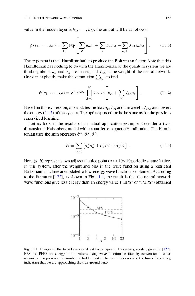
Here a, b represents two adjacent lattice points on a 10×10 periodic square lattice.
In this system, after the weight and bias in the wave function using a restricted
Boltzmann machine are updated, a low-energy wave function is obtained. According
to the literature [122], as shown in Fig. 11.1, the result is that the neural network
wave functions give less energy than an energy value (“EPS” or “PEPS”) obtained
Fig. 11.1 Energy of the two-dimensional antiferromagnetic Heisenberg model, given in [122].
EPS and PEPS are energy minimizations using wave functions written by conventional tensor
networks. α represents the number of hidden units. The more hidden units, the lower the energy,
indicating that we are approaching the true ground state
167
value in the hidden layer is h 1 , · · · , h M , the output will be as follows:
ψ(s 1 , · · · , s N ) =
h A
exp
⎡
⎣
a
a a s a +
A
b A h A +
a,A
J aA s a h A
⎤
⎦ .
(11.3)
The exponent is the “Hamiltonian” to produce the Boltzmann factor. Note that this
Hamiltonian has nothing to do with the Hamiltonian of the quantum system we are
thinking about. a a and b A are biases, and J aA is the weight of the neural network.
One can explicitly make the summation
h A
, to find
ψ(s 1 , · · · , s N ) = e
a a a s a
M
A=1
2 cosh
b A +
a
J aA s a
.
(11.4)
Based on this expression, one updates the bias a a , b A and the weight J aA , and lowers
the energy (11.2) of the system. The update procedure is the same as for the previous
supervised learning.
Let us look at the results of an actual application example. Consider a twodimensional Heisenberg model with an antiferromagnetic Hamiltonian. The Hamiltonian uses the spin operators ˆ
σ x , ˆ
σ y , ˆ
σ z ,
H =
a,b
ˆ
σ
x
a ˆ
σ
x
b + ˆ
σ
y
a ˆ
σ
y
b + ˆ
σ
z
a ˆ
σ
z
b
.
(11.5)
Here a, b represents two adjacent lattice points on a 10×10 periodic square lattice.
In this system, after the weight and bias in the wave function using a restricted
Boltzmann machine are updated, a low-energy wave function is obtained. According
to the literature [122], as shown in Fig. 11.1, the result is that the neural network
wave functions give less energy than an energy value (“EPS” or “PEPS”) obtained
Fig. 11.1 Energy of the two-dimensional antiferromagnetic Heisenberg model, given in [122].
EPS and PEPS are energy minimizations using wave functions written by conventional tensor
networks. α represents the number of hidden units. The more hidden units, the lower the energy,
indicating that we are approaching the true ground state