

164
10 Spinglass and Neural Networks
For the last line, we used sgn(x) = x/|x|. In this last line, using
(S i (n + 2) − S i (n)) S i (n + 2) = 0 or 2,
(10.23)
the following has been proven as expected:
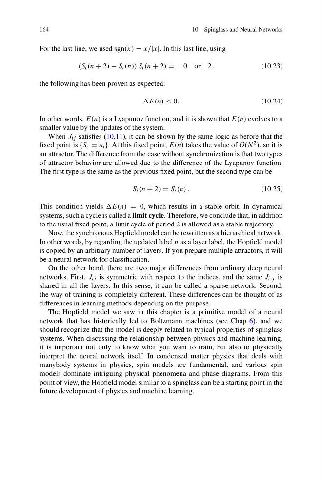
≤ 0.
(10.24)
In other words, E(n) is a Lyapunov function, and it is shown that E(n) evolves to a
smaller value by the updates of the system.
When J ij satisfies (10.11), it can be shown by the same logic as before that the
fixed point is {S i = a i }. At this fixed point, E(n) takes the value of O(N 2 ), so it is
an attractor. The difference from the case without synchronization is that two types
of attractor behavior are allowed due to the difference of the Lyapunov function.
The first type is the same as the previous fixed point, but the second type can be
S i (n + 2) = S i (n) .
(10.25)
This condition yields = 0, which results in a stable orbit. In dynamical
systems, such a cycle is called a limit cycle. Therefore, we conclude that, in addition
to the usual fixed point, a limit cycle of period 2 is allowed as a stable trajectory.
Now, the synchronous Hopfield model can be rewritten as a hierarchical network.
In other words, by regarding the updated label n as a layer label, the Hopfield model
is copied by an arbitrary number of layers. If you prepare multiple attractors, it will
be a neural network for classification.
On the other hand, there are two major differences from ordinary deep neural
networks. First, J ij is symmetric with respect to the indices, and the same J i,j is
shared in all the layers. In this sense, it can be called a sparse network. Second,
the way of training is completely different. These differences can be thought of as
differences in learning methods depending on the purpose.
The Hopfield model we saw in this chapter is a primitive model of a neural
network that has historically led to Boltzmann machines (see Chap. 6), and we
should recognize that the model is deeply related to typical properties of spinglass
systems. When discussing the relationship between physics and machine learning,
it is important not only to know what you want to train, but also to physically
interpret the neural network itself. In condensed matter physics that deals with
manybody systems in physics, spin models are fundamental, and various spin
models dominate intriguing physical phenomena and phase diagrams. From this
point of view, the Hopfield model similar to a spinglass can be a starting point in the
future development of physics and machine learning.
10 Spinglass and Neural Networks
For the last line, we used sgn(x) = x/|x|. In this last line, using
(S i (n + 2) − S i (n)) S i (n + 2) = 0 or 2,
(10.23)
the following has been proven as expected:
≤ 0.
(10.24)
In other words, E(n) is a Lyapunov function, and it is shown that E(n) evolves to a
smaller value by the updates of the system.
When J ij satisfies (10.11), it can be shown by the same logic as before that the
fixed point is {S i = a i }. At this fixed point, E(n) takes the value of O(N 2 ), so it is
an attractor. The difference from the case without synchronization is that two types
of attractor behavior are allowed due to the difference of the Lyapunov function.
The first type is the same as the previous fixed point, but the second type can be
S i (n + 2) = S i (n) .
(10.25)
This condition yields = 0, which results in a stable orbit. In dynamical
systems, such a cycle is called a limit cycle. Therefore, we conclude that, in addition
to the usual fixed point, a limit cycle of period 2 is allowed as a stable trajectory.
Now, the synchronous Hopfield model can be rewritten as a hierarchical network.
In other words, by regarding the updated label n as a layer label, the Hopfield model
is copied by an arbitrary number of layers. If you prepare multiple attractors, it will
be a neural network for classification.
On the other hand, there are two major differences from ordinary deep neural
networks. First, J ij is symmetric with respect to the indices, and the same J i,j is
shared in all the layers. In this sense, it can be called a sparse network. Second,
the way of training is completely different. These differences can be thought of as
differences in learning methods depending on the purpose.
The Hopfield model we saw in this chapter is a primitive model of a neural
network that has historically led to Boltzmann machines (see Chap. 6), and we
should recognize that the model is deeply related to typical properties of spinglass
systems. When discussing the relationship between physics and machine learning,
it is important not only to know what you want to train, but also to physically
interpret the neural network itself. In condensed matter physics that deals with
manybody systems in physics, spin models are fundamental, and various spin
models dominate intriguing physical phenomena and phase diagrams. From this
point of view, the Hopfield model similar to a spinglass can be a starting point in the
future development of physics and machine learning.