

6.3 Generative Adversarial Network
111
can be regarded as a variational problem in physics, to seek for a solution of the
equation
0 =
δV D (G, D)
δD(x)
.
(6.43)
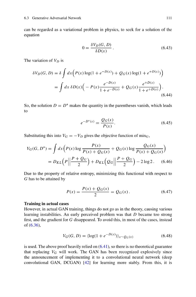
The variation of V D is
δV D (G, D) = δ
dx
P (x) log(1 + e
−D(x) ) + Q G (x) log(1 + e
+D(x) )
=
dx δD(x)
− P (x)
e −D(x)
1 + e −D(x) + Q G (x)
e +D(x)
1 + e +D(x)
.
(6.44)
So, the solution D = D ∗ makes the quantity in the parentheses vanish, which leads
to
e
−D ∗ (x)
=
Q G (x)
P (x)
.
(6.45)
Substituting this into V G = −V D gives the objective function of min G ,
V G (G, D
∗ ) =
dx
P (x) log
P (x)
P (x) + Q G (x)
+ Q G (x) log
Q G (x)
P (x) + Q G (x)
= D KL
P
P + Q G
2
+ D KL
Q G
P + Q G
2
− 2 log 2 .
(6.46)
Due to the property of relative entropy, minimizing this functional with respect to
G has to be attained by
P (x) =
P (x) + Q G (x)
2
= Q G (x) .
(6.47)
Training in actual cases
However, in actual GAN training, things do not go as in the theory, causing various
learning instabilities. An early perceived problem was that D became too strong
first, and the gradient for G disappeared. To avoid this, in most of the cases, instead
of (6.36),
V G (G, D) = =log(1 + e
−D(x) ) x∼Q G (x)
(6.48)
is used. The above proof heavily relied on (6.41), so there is no theoretical guarantee
that replacing V G will work. The GAN has been recognized explosively since
the announcement of implementing it to a convolutional neural network (deep
convolutional GAN, DCGAN) [42] for learning more stably. From this, it is
111
can be regarded as a variational problem in physics, to seek for a solution of the
equation
0 =
δV D (G, D)
δD(x)
.
(6.43)
The variation of V D is
δV D (G, D) = δ
dx
P (x) log(1 + e
−D(x) ) + Q G (x) log(1 + e
+D(x) )
=
dx δD(x)
− P (x)
e −D(x)
1 + e −D(x) + Q G (x)
e +D(x)
1 + e +D(x)
.
(6.44)
So, the solution D = D ∗ makes the quantity in the parentheses vanish, which leads
to
e
−D ∗ (x)
=
Q G (x)
P (x)
.
(6.45)
Substituting this into V G = −V D gives the objective function of min G ,
V G (G, D
∗ ) =
dx
P (x) log
P (x)
P (x) + Q G (x)
+ Q G (x) log
Q G (x)
P (x) + Q G (x)
= D KL
P
P + Q G
2
+ D KL
Q G
P + Q G
2
− 2 log 2 .
(6.46)
Due to the property of relative entropy, minimizing this functional with respect to
G has to be attained by
P (x) =
P (x) + Q G (x)
2
= Q G (x) .
(6.47)
Training in actual cases
However, in actual GAN training, things do not go as in the theory, causing various
learning instabilities. An early perceived problem was that D became too strong
first, and the gradient for G disappeared. To avoid this, in most of the cases, instead
of (6.36),
V G (G, D) = =log(1 + e
−D(x) ) x∼Q G (x)
(6.48)
is used. The above proof heavily relied on (6.41), so there is no theoretical guarantee
that replacing V G will work. The GAN has been recognized explosively since
the announcement of implementing it to a convolutional neural network (deep
convolutional GAN, DCGAN) [42] for learning more stably. From this, it is