

3.4 Solved Problems
69
Evaluation of the finite difference approximation of the second-order differential
equation according to Eq. (3.143) at the nodes i = 1, . . . , 6 gives
7 :
node 1:
E I Y
X 2 (u 2 − 2u 1 + u 0 ) = −F 0 L ,
(3.145)
node 2:
E I Y
X 2 (u 3 − 2u 2 + u 1 ) = −
5F 0 L
6
,
(3.146)
node 3:
E I Y
X 2 (u 4 − 2u 3 + u 2 ) = −
4F 0 L
6
,
(3.147)
node 4:
E I Y
X 2 (u 5 − 2u 4 + u 3 ) = −
3F 0 L
6
,
(3.148)
node 5:
E I Y
X 2 (u 6 − 2u 5 + u 4 ) = −
2F 0 L
6
,
(3.149)
node 6:
E I Y
X 2 (u 7 − 2u 6 + u 5 ) = −
1F 0 L
6
,
(3.150)
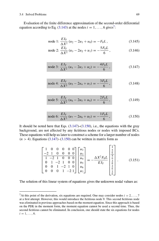
It should be noted here that Eqs. (3.147)–(3.150), i.e., the equations with the gray
background, are not affected by any fictitious nodes or nodes with imposed BCs.
These equations will help us later to construct a scheme for a larger number of nodes
(n > 4). Equations (3.147)–(3.150) can be written in matrix form as
⎡
⎢
⎢
⎢
⎢
⎢
⎢
⎣
1 0 0 0 0 0
−2 1 0 0 0 0
1 −2 1 0 0 0
0 1 −2 1 0 0
0 0 1 −2 1 0
0 0 0 1 −2 1
⎤
⎥
⎥
⎥
⎥
⎥
⎥
⎦
⎡
⎢
⎢
⎢
⎢
⎢
⎢
⎣
u 2
u 3
u 4
u 5
u 6
u 7
⎤
⎥
⎥
⎥
⎥
⎥
⎥
⎦
= −
X
2 F 0 L
E I Y
⎡
⎢
⎢
⎢
⎢
⎢
⎢
⎢
⎢
⎣
1
5
6
4
6
3
6
2
6
1
6
⎤
⎥
⎥
⎥
⎥
⎥
⎥
⎥
⎥
⎦
.
(3.151)
The solution of this linear system of equations gives the unknown nodal values as:
7 At this point of the derivation, six equations are required. One may consider nodes i = 2, . . . , 7
at a first attempt. However, this would introduce the fictitious node 9. This second fictitious node
was eliminated in previous approaches based on the moment equation. Since this approach is based
on the PDE in the moment form, the moment equation cannot be used a second time. Thus, the
second fictitious cannot be eliminated. In conclusion, one should state the six equations for nodes
i = 1, . . . , 6.
69
Evaluation of the finite difference approximation of the second-order differential
equation according to Eq. (3.143) at the nodes i = 1, . . . , 6 gives
7 :
node 1:
E I Y
X 2 (u 2 − 2u 1 + u 0 ) = −F 0 L ,
(3.145)
node 2:
E I Y
X 2 (u 3 − 2u 2 + u 1 ) = −
5F 0 L
6
,
(3.146)
node 3:
E I Y
X 2 (u 4 − 2u 3 + u 2 ) = −
4F 0 L
6
,
(3.147)
node 4:
E I Y
X 2 (u 5 − 2u 4 + u 3 ) = −
3F 0 L
6
,
(3.148)
node 5:
E I Y
X 2 (u 6 − 2u 5 + u 4 ) = −
2F 0 L
6
,
(3.149)
node 6:
E I Y
X 2 (u 7 − 2u 6 + u 5 ) = −
1F 0 L
6
,
(3.150)
It should be noted here that Eqs. (3.147)–(3.150), i.e., the equations with the gray
background, are not affected by any fictitious nodes or nodes with imposed BCs.
These equations will help us later to construct a scheme for a larger number of nodes
(n > 4). Equations (3.147)–(3.150) can be written in matrix form as
⎡
⎢
⎢
⎢
⎢
⎢
⎢
⎣
1 0 0 0 0 0
−2 1 0 0 0 0
1 −2 1 0 0 0
0 1 −2 1 0 0
0 0 1 −2 1 0
0 0 0 1 −2 1
⎤
⎥
⎥
⎥
⎥
⎥
⎥
⎦
⎡
⎢
⎢
⎢
⎢
⎢
⎢
⎣
u 2
u 3
u 4
u 5
u 6
u 7
⎤
⎥
⎥
⎥
⎥
⎥
⎥
⎦
= −
X
2 F 0 L
E I Y
⎡
⎢
⎢
⎢
⎢
⎢
⎢
⎢
⎢
⎣
1
5
6
4
6
3
6
2
6
1
6
⎤
⎥
⎥
⎥
⎥
⎥
⎥
⎥
⎥
⎦
.
(3.151)
The solution of this linear system of equations gives the unknown nodal values as:
7 At this point of the derivation, six equations are required. One may consider nodes i = 2, . . . , 7
at a first attempt. However, this would introduce the fictitious node 9. This second fictitious node
was eliminated in previous approaches based on the moment equation. Since this approach is based
on the PDE in the moment form, the moment equation cannot be used a second time. Thus, the
second fictitious cannot be eliminated. In conclusion, one should state the six equations for nodes
i = 1, . . . , 6.