

3.4 Solved Problems
67
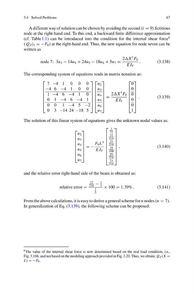
A different way of solution can be chosen by avoiding the second (i = 9) fictitious
node at the right-hand end. To this end, a backward finite difference approximation
(cf. Table 1.1) can be introduced into the condition for the internal shear force
6
( Q Z | 7 = −F 0 ) at the right-hand end. Thus, the new equation for node seven can be
written as
node 7: 3u 3 − 14u 4 + 24u 5 − 18u 6 + 5u 7 =
2X
3 F 0
E I Y
.
(3.138)
The corresponding system of equations reads in matrix notation as:
⎡
⎢
⎢
⎢
⎢
⎢
⎢
⎣
7 −4 1 0 0 0
−4 6 −4 1 0 0
1 −4 6 −4 1 0
0 1 −4 6 −4 1
0 0 1 −4 5 −2
0 3 −14 24 −18 5
⎤
⎥
⎥
⎥
⎥
⎥
⎥
⎦
⎡
⎢
⎢
⎢
⎢
⎢
⎢
⎣
u 2
u 3
u 4
u 5
u 6
u 7
⎤
⎥
⎥
⎥
⎥
⎥
⎥
⎦
=
2X
3 F 0
E I Y
⎡
⎢
⎢
⎢
⎢
⎢
⎢
⎣
0
0
0
0
0
1
⎤
⎥
⎥
⎥
⎥
⎥
⎥
⎦
.
(3.139)
The solution of this linear system of equations gives the unknown nodal values as:
⎡
⎢
⎢
⎢
⎢
⎢
⎢
⎣
u 2
u 3
u 4
u 5
u 6
u 7
⎤
⎥
⎥
⎥
⎥
⎥
⎥
⎦
= −
F 0 L
3
E I Y
⎡
⎢
⎢
⎢
⎢
⎢
⎢
⎢
⎢
⎣
1
72
11
216
23
216
19
108
55
216
73
216
⎤
⎥
⎥
⎥
⎥
⎥
⎥
⎥
⎥
⎦
,
(3.140)
and the relative error right-hand side of the beam is obtained as:
relative error =
73
216
−
1
3
1
3
× 100 = 1.39% .
(3.141)
From the above calculations, it is easy to derive a general scheme for n nodes (n > 7).
In generalization of Eq. (3.139), the following scheme can be proposed:
6 The value of the internal shear force is now determined based on the real load condition, i.e.,
Fig. 3.16b, and not based on the modeling approach provided in Fig. 3.20. Thus, we obtain: Q Z (X =
L) = −F 0 .
67
A different way of solution can be chosen by avoiding the second (i = 9) fictitious
node at the right-hand end. To this end, a backward finite difference approximation
(cf. Table 1.1) can be introduced into the condition for the internal shear force
6
( Q Z | 7 = −F 0 ) at the right-hand end. Thus, the new equation for node seven can be
written as
node 7: 3u 3 − 14u 4 + 24u 5 − 18u 6 + 5u 7 =
2X
3 F 0
E I Y
.
(3.138)
The corresponding system of equations reads in matrix notation as:
⎡
⎢
⎢
⎢
⎢
⎢
⎢
⎣
7 −4 1 0 0 0
−4 6 −4 1 0 0
1 −4 6 −4 1 0
0 1 −4 6 −4 1
0 0 1 −4 5 −2
0 3 −14 24 −18 5
⎤
⎥
⎥
⎥
⎥
⎥
⎥
⎦
⎡
⎢
⎢
⎢
⎢
⎢
⎢
⎣
u 2
u 3
u 4
u 5
u 6
u 7
⎤
⎥
⎥
⎥
⎥
⎥
⎥
⎦
=
2X
3 F 0
E I Y
⎡
⎢
⎢
⎢
⎢
⎢
⎢
⎣
0
0
0
0
0
1
⎤
⎥
⎥
⎥
⎥
⎥
⎥
⎦
.
(3.139)
The solution of this linear system of equations gives the unknown nodal values as:
⎡
⎢
⎢
⎢
⎢
⎢
⎢
⎣
u 2
u 3
u 4
u 5
u 6
u 7
⎤
⎥
⎥
⎥
⎥
⎥
⎥
⎦
= −
F 0 L
3
E I Y
⎡
⎢
⎢
⎢
⎢
⎢
⎢
⎢
⎢
⎣
1
72
11
216
23
216
19
108
55
216
73
216
⎤
⎥
⎥
⎥
⎥
⎥
⎥
⎥
⎥
⎦
,
(3.140)
and the relative error right-hand side of the beam is obtained as:
relative error =
73
216
−
1
3
1
3
× 100 = 1.39% .
(3.141)
From the above calculations, it is easy to derive a general scheme for n nodes (n > 7).
In generalization of Eq. (3.139), the following scheme can be proposed:
6 The value of the internal shear force is now determined based on the real load condition, i.e.,
Fig. 3.16b, and not based on the modeling approach provided in Fig. 3.20. Thus, we obtain: Q Z (X =
L) = −F 0 .