

58
3 Investigation of Euler–Bernoulli Beams in the Elastic Range
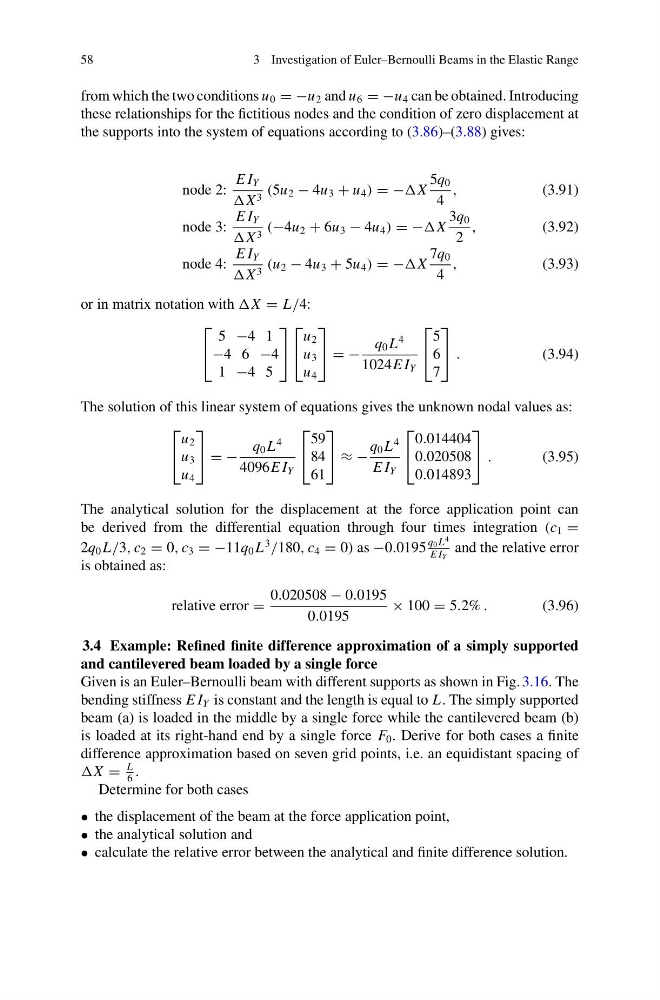
from which the two conditions u 0 = −u 2 and u 6 = −u 4 can be obtained. Introducing
these relationships for the fictitious nodes and the condition of zero displacement at
the supports into the system of equations according to (3.86)–(3.88) gives:
node 2:
E I Y
X 3 (5u 2 − 4u 3 + u 4 ) = −X
5q 0
4
,
(3.91)
node 3:
E I Y
X 3 (−4u 2 + 6u 3 − 4u 4 ) = −X
3q 0
2
,
(3.92)
node 4:
E I Y
X 3 (u 2 − 4u 3 + 5u 4 ) = −X
7q 0
4
,
(3.93)
or in matrix notation with X = L/4:
⎡
⎣
5 −4 1
−4 6 −4
1 −4 5
⎤
⎦
⎡
⎣
u 2
u 3
u 4
⎤
⎦ = −
q 0 L
4
1024E I Y
⎡
⎣
5
6
7
⎤
⎦ .
(3.94)
The solution of this linear system of equations gives the unknown nodal values as:
⎡
⎣
u 2
u 3
u 4
⎤
⎦ = −
q 0 L
4
4096E I Y
⎡
⎣
59
84
61
⎤
⎦ ≈ −
q 0 L
4
E I Y
⎡
⎣
0.014404
0.020508
0.014893
⎤
⎦ .
(3.95)
The analytical solution for the displacement at the force application point can
be derived from the differential equation through four times integration (c 1 =
2q 0 L/3, c 2 = 0, c 3 = −11q 0 L
3
/180, c 4 = 0) as −0.0195
q 0 L
4
E I Y
and the relative error
is obtained as:
relative error =
0.020508 − 0.0195
0.0195
× 100 = 5.2% .
(3.96)
3.4 Example: Refined finite difference approximation of a simply supported
and cantilevered beam loaded by a single force
Given is an Euler–Bernoulli beam with different supports as shown in Fig. 3.16. The
bending stiffness E I Y is constant and the length is equal to L. The simply supported
beam (a) is loaded in the middle by a single force while the cantilevered beam (b)
is loaded at its right-hand end by a single force F 0 . Derive for both cases a finite
difference approximation based on seven grid points, i.e. an equidistant spacing of
X =
L
6
.
Determine for both cases
• the displacement of the beam at the force application point,
• the analytical solution and
• calculate the relative error between the analytical and finite difference solution.
3 Investigation of Euler–Bernoulli Beams in the Elastic Range
from which the two conditions u 0 = −u 2 and u 6 = −u 4 can be obtained. Introducing
these relationships for the fictitious nodes and the condition of zero displacement at
the supports into the system of equations according to (3.86)–(3.88) gives:
node 2:
E I Y
X 3 (5u 2 − 4u 3 + u 4 ) = −X
5q 0
4
,
(3.91)
node 3:
E I Y
X 3 (−4u 2 + 6u 3 − 4u 4 ) = −X
3q 0
2
,
(3.92)
node 4:
E I Y
X 3 (u 2 − 4u 3 + 5u 4 ) = −X
7q 0
4
,
(3.93)
or in matrix notation with X = L/4:
⎡
⎣
5 −4 1
−4 6 −4
1 −4 5
⎤
⎦
⎡
⎣
u 2
u 3
u 4
⎤
⎦ = −
q 0 L
4
1024E I Y
⎡
⎣
5
6
7
⎤
⎦ .
(3.94)
The solution of this linear system of equations gives the unknown nodal values as:
⎡
⎣
u 2
u 3
u 4
⎤
⎦ = −
q 0 L
4
4096E I Y
⎡
⎣
59
84
61
⎤
⎦ ≈ −
q 0 L
4
E I Y
⎡
⎣
0.014404
0.020508
0.014893
⎤
⎦ .
(3.95)
The analytical solution for the displacement at the force application point can
be derived from the differential equation through four times integration (c 1 =
2q 0 L/3, c 2 = 0, c 3 = −11q 0 L
3
/180, c 4 = 0) as −0.0195
q 0 L
4
E I Y
and the relative error
is obtained as:
relative error =
0.020508 − 0.0195
0.0195
× 100 = 5.2% .
(3.96)
3.4 Example: Refined finite difference approximation of a simply supported
and cantilevered beam loaded by a single force
Given is an Euler–Bernoulli beam with different supports as shown in Fig. 3.16. The
bending stiffness E I Y is constant and the length is equal to L. The simply supported
beam (a) is loaded in the middle by a single force while the cantilevered beam (b)
is loaded at its right-hand end by a single force F 0 . Derive for both cases a finite
difference approximation based on seven grid points, i.e. an equidistant spacing of
X =
L
6
.
Determine for both cases
• the displacement of the beam at the force application point,
• the analytical solution and
• calculate the relative error between the analytical and finite difference solution.